Este artículo tiene varios problemas. Ayude a mejorarlo o discuta estos problemas en la página de discusión . ( Obtenga información sobre cómo y cuándo eliminar estos mensajes de plantilla ) ( Aprenda cómo y cuándo eliminar este mensaje de plantilla )
|
| Más allá del modelo estándar |
|---|
 |
| Modelo estandar |
La gravedad cuántica de bucle ( LQG ) [1] [2] [3] [4] [5] es una teoría de la gravedad cuántica , que tiene como objetivo fusionar la mecánica cuántica y la relatividad general , incorporando materia del Modelo Estándar en el marco establecido para el caso de gravedad cuántica pura. Como candidato a la gravedad cuántica, LQG compite con la teoría de cuerdas . [6]
La gravedad cuántica de bucle es un intento de desarrollar una teoría cuántica de la gravedad basada directamente en la formulación geométrica de Einstein en lugar del tratamiento de la gravedad como una fuerza. Para hacer esto, en la teoría LQG, el espacio y el tiempo se cuantifican de manera análoga a la forma en que cantidades como la energía y el momento se cuantifican en la mecánica cuántica . La teoría da una imagen física del espacio-tiempo donde el espacio y el tiempo son granulares y discretos directamente debido a la cuantificación al igual que los fotones en la teoría cuántica del electromagnetismo y los niveles de energía discretos de los átomos . Una implicación de un espacio cuantificado es que existe una distancia mínima.
LQG postula que la estructura del espacio se compone de bucles finitos tejidos en una tela o red extremadamente fina. Estas redes de bucles se denominan redes giratorias . La evolución de una red de espín, o espuma de espín , tiene una escala del orden de una longitud de Planck , aproximadamente de 10 a 35 metros, y las escalas más pequeñas no tienen sentido. En consecuencia, no solo la materia, sino el espacio mismo, prefiere una estructura atómica .
Las áreas de investigación, que involucran a unos 30 grupos de investigación en todo el mundo, [7] comparten los supuestos físicos básicos y la descripción matemática del espacio cuántico. La investigación ha evolucionado en dos direcciones: la gravedad cuántica de bucle canónico más tradicional y la gravedad cuántica de bucle covariante más reciente, llamada teoría de la espuma de espín .
La teoría más desarrollada que se ha propuesto como resultado directo de la gravedad cuántica de bucles se denomina cosmología cuántica de bucles (LQC). LQC avanza en el estudio del universo temprano, incorporando el concepto del Big Bang en la teoría más amplia del Big Bounce , que visualiza el Big Bang como el comienzo de un período de expansión que sigue a un período de contracción, del que se podría hablar. como el Big Crunch .
Historia [ editar ]
En 1986, Abhay Ashtekar reformuló la relatividad general de Einstein en un lenguaje más cercano al del resto de la física fundamental. [ cita requerida ] Poco después, Ted Jacobson y Lee Smolin se dieron cuenta de que la ecuación formal de la gravedad cuántica, llamada ecuación de Wheeler-DeWitt , admitía soluciones etiquetadas con bucles cuando se reescribían en las nuevas variables de Ashtekar . Carlo Rovelli y Smolin definieron una teoría cuántica de la gravedad no perturbativa e independiente del fondo en términos de estas soluciones de bucle. Jorge Pulliny Jerzy Lewandowski entendió que las intersecciones de los bucles son esenciales para la coherencia de la teoría, y la teoría debe formularse en términos de bucles o gráficos que se cruzan .
En 1994, Rovelli y Smolin demostraron que los operadores cuánticos de la teoría asociados al área y al volumen tienen un espectro discreto. Es decir, la geometría se cuantifica. Este resultado define una base explícita de estados de geometría cuántica, que resultaron estar etiquetados por las redes de espines de Roger Penrose , que son gráficos etiquetados por espines .
La versión canónica de la dinámica fue establecida por Thomas Thiemann, quien definió un operador hamiltoniano libre de anomalías y mostró la existencia de una teoría independiente del trasfondo matemáticamente consistente. La versión covariante, o " espuma de hilado ", de la dinámica fue desarrollada conjuntamente durante varias décadas por grupos de investigación en Francia, Canadá, Reino Unido, Polonia y Alemania. Se completó en 2008, dando lugar a la definición de una familia de amplitudes de transición, que en el límite clásico se puede demostrar que está relacionada con una familia de truncamientos de la relatividad general. [8] La finitud de estas amplitudes se demostró en 2011. [9] [10] Requiere la existencia de una constante cosmológica positiva, que es consistente con la aceleración observada en la expansión del Universo .
Covarianza general e independencia de fondo [ editar ]
En física teórica, la covarianza general es la invariancia de la forma de las leyes físicas bajo transformaciones de coordenadas diferenciables arbitrarias. La idea esencial es que las coordenadas son sólo artificios que se utilizan para describir la naturaleza y, por tanto, no deberían desempeñar ningún papel en la formulación de las leyes físicas fundamentales. Un requisito más significativo es el principio de relatividad general que establece que las leyes de la física toman la misma forma en todos los sistemas de referencia. Esta es una generalización del principio de relatividad especial que establece que las leyes de la física toman la misma forma en todos los marcos inerciales.
En matemáticas, un difeomorfismo es un isomorfismo en la categoría de variedades suaves. Es una función invertible que mapea una variedad diferenciable a otra, de modo que tanto la función como su inversa son suaves. Estas son las transformaciones de simetría definitorias de la Relatividad General, ya que la teoría se formula solo en términos de una variedad diferenciable.
En la relatividad general, la covarianza general está íntimamente relacionada con la "invariancia de difeomorfismo". Esta simetría es una de las características definitorias de la teoría. Sin embargo, es un malentendido común que la "invariancia de difeomorfismo" se refiere a la invariancia de las predicciones físicas de una teoría bajo transformaciones de coordenadas arbitrarias ; esto es falso y, de hecho, toda teoría física es invariante bajo transformaciones de coordenadas de esta manera. Los difeomorfismos , como los definen los matemáticos, corresponden a algo mucho más radical; intuitivamente, una forma en que se pueden imaginar es arrastrando simultáneamente todos los campos físicos (incluido el campo gravitacional) sobre la variedad diferenciable desnudamientras permanece en el mismo sistema de coordenadas. Los difeomorfismos son las verdaderas transformaciones de simetría de la relatividad general, y surgen de la afirmación de que la formulación de la teoría se basa en una variedad diferenciable pura, pero no en ninguna geometría previa: la teoría es independiente del fondo.(este es un cambio profundo, ya que todas las teorías físicas anteriores a la relatividad general tenían como parte de su formulación una geometría previa). Lo que se conserva bajo tales transformaciones son las coincidencias entre los valores que el campo gravitacional toma en tal o cual "lugar" y los valores que los campos de materia toman allí. A partir de estas relaciones, se puede formar una noción de que la materia está ubicada con respecto al campo gravitacional, o viceversa. Esto es lo que descubrió Einstein: que las entidades físicas están ubicadas entre sí solamente y no con respecto a la variedad espacio-tiempo. Como dice Carlo Rovelli : "No más campos en el espacio-tiempo: solo campos en los campos". [11]Este es el verdadero significado del dicho "El escenario desaparece y se convierte en uno de los actores"; el espacio-tiempo como un "contenedor" sobre el que tiene lugar la física no tiene un significado físico objetivo y, en cambio, la interacción gravitacional se representa como uno de los campos que forman el mundo. Esto se conoce como la interpretación relacionalista del espacio-tiempo. La comprensión por parte de Einstein de que la relatividad general debe interpretarse de esta manera es el origen de su comentario "Más allá de mis expectativas más salvajes".
En LQG, este aspecto de la relatividad general se toma en serio y esta simetría se conserva al exigir que los estados físicos permanezcan invariantes bajo los generadores de difeomorfismos. La interpretación de esta condición es bien conocida para difeomorfismos puramente espaciales. Sin embargo, la comprensión de los difeomorfismos que involucran el tiempo (la restricción hamiltoniana ) es más sutil porque está relacionada con la dinámica y el llamado " problema del tiempo " en la relatividad general. [12] Aún no se ha encontrado un marco de cálculo generalmente aceptado para tener en cuenta esta restricción. [13] [14] Un candidato plausible para la restricción cuántica hamiltoniana es el operador introducido por Thiemann. [15]
LQG es formalmente independiente de antecedentes . Las ecuaciones de LQG no están integradas ni dependen del espacio y el tiempo (excepto por su topología invariante). En cambio, se espera que den lugar al espacio y al tiempo a distancias que son 10 veces la longitud de Planck . El tema de la independencia de fondo en LQG todavía tiene algunas sutilezas sin resolver. Por ejemplo, algunas derivaciones requieren una elección fija de la topología , mientras que cualquier teoría cuántica de la gravedad consistente debería incluir el cambio de topología como un proceso dinámico.
Restricciones y su álgebra de corchetes de Poisson [ editar ]
Las limitaciones de la relatividad general canónica clásica [ editar ]
La relatividad general es un ejemplo de un sistema restringido. En la formulación hamiltoniana de la mecánica clásica ordinaria, el corchete de Poisson es un concepto importante. Un "sistema de coordenadas canónico" consta de variables canónicas de posición y momento que satisfacen las relaciones canónicas entre paréntesis de Poisson,

donde el corchete de Poisson viene dado por

para funciones de espacio de fase arbitrarias y . Con el uso de corchetes de Poisson, las ecuaciones de Hamilton se pueden reescribir como,


Estas ecuaciones describen un " flujo " u órbita en el espacio de fase generado por el hamiltoniano . Dada cualquier función de espacio de fase , produce


De manera similar, el corchete de Poisson entre una restricción y las variables de espacio de fase genera un flujo a lo largo de una órbita en el espacio de fase (no restringido) generado por la restricción. Hay tres tipos de restricciones en la reformulación de Ashtekar de la relatividad general clásica:
SU (2) Restricciones de calibre de Gauss [ editar ]
Las limitaciones de Gauss

Esto representa un número infinito de restricciones, una por cada valor de . Estos surgen de la reexpresión de la relatividad general como una teoría gauge de tipo Yang-Mills (Yang-Mills es una generalización de la teoría de Maxwell donde el campo gauge se transforma como un vector bajo las transformaciones de Gauss, es decir, el campo Gauge tiene la forma donde es un índice interno (ver variables Ashtekar ). Este número infinito de restricciones de calibre de Gauss puede ser " manchado " por campos de prueba con índices internos ,


que debe desaparecer para tal función. Estas restricciones difusas definidas con respecto a un espacio adecuado de funciones de difuminado dan una descripción equivalente a las restricciones originales.
La formulación de Ashtekar se puede considerar como la teoría de Yang-Mills ordinaria junto con las siguientes restricciones especiales, resultantes de la invariancia de difeomorfismo, y un hamiltoniano que se desvanece. La dinámica de tal teoría es, por tanto, muy diferente de la de la teoría ordinaria de Yang-Mills.
Restricciones de difeomorfismos espaciales [ editar ]
Las limitaciones del difeomorfismo espacial

puede ser difuminado por las llamadas funciones de desplazamiento para dar un conjunto equivalente de restricciones de difeomorfismo espacial difuminado,


Estos generan difeomorfismos espaciales a lo largo de órbitas definidas por la función de desplazamiento .

Restricciones hamiltonianas [ editar ]
El hamiltoniano

se puede difuminar por las llamadas funciones de lapso para dar un conjunto equivalente de restricciones hamiltonianas difuminadas,

- .

Estos generan difeomorfismos de tiempo a lo largo de órbitas definidas por la función de lapso .
En la formulación de Ashtekar, el campo gauge es la variable de configuración (la variable de configuración es análoga a la de la mecánica ordinaria) y su momento conjugado es la tríada (densitizada) (campo eléctrico) . Las restricciones son ciertas funciones de estas variables de espacio de fase.


Un aspecto importante de la acción de las limitaciones de espacio funciona de fase arbitrario es la derivada de Lie , , que es básicamente una operación de derivado que infinitesimalmente funciones "desplaza" a lo largo de algunos órbita con vector tangente .


Observables de Dirac [ editar ]
Las restricciones definen una superficie de restricción en el espacio de fase original. Los movimientos de calibre de las restricciones se aplican a todo el espacio de fase pero tienen la característica de que dejan la superficie de restricción donde está y, por lo tanto, la órbita de un punto en la hipersuperficie bajo transformaciones de calibre será una órbita completamente dentro de ella. Los observables de Dirac se definen como funciones de espacio de fase , que Poisson conmuta con todas las restricciones cuando se imponen las ecuaciones de restricción,

- ,

es decir, son cantidades definidas en la superficie de restricción que son invariantes bajo las transformaciones de calibre de la teoría.
Entonces, resolver solo la restricción y determinar los observables de Dirac con respecto a ella nos lleva de regreso al espacio de fase de Arnowitt-Deser-Misner (ADM) con restricciones . La dinámica de la relatividad general es generada por las restricciones, se puede demostrar que seis ecuaciones de Einstein que describen la evolución del tiempo (en realidad una transformación de indicador) se pueden obtener calculando los paréntesis de Poisson de la métrica de tres y su momento conjugado con una combinación lineal de el difeomorfismo espacial y la restricción hamiltoniana. La desaparición de las restricciones, dando el espacio de fase física, son las otras cuatro ecuaciones de Einstein. [dieciséis]


Cuantización de las restricciones: las ecuaciones de la relatividad general cuántica [ editar ]
Prehistoria y nuevas variables de Ashtekar [ editar ]
Muchos de los problemas técnicos de la gravedad cuántica canónica giran en torno a las limitaciones. La relatividad general canónica se formuló originalmente en términos de variables métricas, pero parecía haber dificultades matemáticas insuperables para promover las restricciones a los operadores cuánticos debido a su dependencia altamente no lineal de las variables canónicas. Las ecuaciones se simplificaron mucho con la introducción de las nuevas variables de Ashtekar. Las variables de Ashtekar describen la relatividad general canónica en términos de un nuevo par de variables canónicas más cercanas a las de las teorías de gauge. El primer paso consiste en utilizar tríadas densitizadas (una tríada es simplemente tres campos vectoriales ortogonales etiquetados por y la tríada densitizada está definida por) para codificar información sobre la métrica espacial,


- .

(donde es la métrica del espacio plano, y la ecuación anterior expresa que , cuando se escribe en términos de la base , es localmente plano). (No era nuevo formular la relatividad general con tríadas en lugar de métricas). Las tríadas densitizadas no son únicas y, de hecho, se puede realizar una rotación local en el espacio con respecto a los índices internos . La variable conjugada canónicamente está relacionada con la curvatura extrínseca por . Pero surgen problemas similares al uso de la formulación métrica cuando se intenta cuantificar la teoría. La nueva visión de Ashtekar fue introducir una nueva variable de configuración,


que se comporta como una conexión compleja donde se relaciona con la llamada conexión de espín vía . Aquí se llama conexión de espín quiral. Define una derivada covariante . Resulta que es el momento conjugado de , y juntos forman las nuevas variables de Ashtekar.


Las expresiones para las restricciones en las variables Ashtekar; la ley de Gauss, la restricción de difeomorfismo espacial y la restricción hamiltoniana (densitizada) entonces leen:

- ,


respectivamente, donde es el tensor de intensidad de campo de la conexión y donde se denomina restricción vectorial. La invariancia rotacional local en el espacio mencionada anteriormente es el original de la invariancia de calibre aquí expresada por la ley de Gauss. Tenga en cuenta que estas restricciones son polinomiales en las variables fundamentales, a diferencia de las restricciones en la formulación métrica. Esta dramática simplificación pareció abrir el camino para cuantificar las limitaciones. (Ver el artículo Acción Palatini auto-dual para una derivación del formalismo de Ashtekar).


Con las nuevas variables de Ashtekar, dada la variable de configuración , es natural considerar las funciones de onda . Esta es la representación de la conexión. Es análogo a la mecánica cuántica ordinaria con variables de configuración y funciones de onda . La variable de configuración se promueve a un operador cuántico a través de:


(análogo a ) y las tríadas son derivados (funcionales),

- .

(análogo a ). Al pasar a la teoría cuántica, las restricciones se convierten en operadores en un espacio cinemático de Hilbert (el espacio sin restricciones de Yang-Mills Hilbert). Tenga en cuenta que el orden diferente de las 'sy ' cuando se reemplazan las 's por derivadas da lugar a operadores diferentes; la elección realizada se denomina ordenación de factores y debe elegirse mediante el razonamiento físico. Formalmente ellos leen


- .

Todavía existen problemas para definir correctamente todas estas ecuaciones y resolverlas. Por ejemplo, la restricción hamiltoniana con la que trabajó Ashtekar fue la versión densitizada en lugar de la hamiltoniana original, es decir, con la que trabajó . Hubo serias dificultades para promover esta cantidad a un operador cuántico. Además, aunque las variables de Ashtekar tenían la virtud de simplificar el hamiltoniano, son complejas. Cuando se cuantifica la teoría, es difícil asegurar que se recupere la relatividad general real en oposición a la relatividad general compleja.

Restricciones cuánticas como ecuaciones de la relatividad general cuántica [ editar ]
El resultado clásico del corchete de Poisson de la ley de Gauss difuminada con las conexiones es


La ley cuántica de Gauss dice
![{\hat {G}}_{j}\Psi (A)=-iD_{a}{\delta \lambda \Psi [A] \over \delta A_{a}^{j}}=0.](https://wikimedia.org/api/rest_v1/media/math/render/svg/60ce26223748ffe84f2065569958e77d7dfb1c17)
Si uno difumina la ley cuántica de Gauss y estudia su acción sobre el estado cuántico, se encuentra que la acción de la restricción sobre el estado cuántico es equivalente a cambiar el argumento de por una transformación de calibre infinitesimal (en el sentido del parámetro pequeño),


![{\displaystyle \left[1+\int d^{3}x\lambda ^{j}(x){\hat {G}}_{j}\right]\Psi (A)=\Psi [A+D\lambda ]=\Psi [A],}](https://wikimedia.org/api/rest_v1/media/math/render/svg/08fa4f29b3c28c30e2be1b0664f40bb73bb27b2c)
y la última identidad proviene del hecho de que la restricción aniquila al estado. Entonces, la restricción, como operador cuántico, está imponiendo la misma simetría que su desaparición imponía clásicamente: nos está diciendo que las funciones tienen que ser funciones invariantes de calibre de la conexión. La misma idea es válida para las otras restricciones.
![\Psi [A]](https://wikimedia.org/api/rest_v1/media/math/render/svg/67ff914baeb5bd928ed9ccd89572a317f07999d3)
Por lo tanto, el proceso de dos pasos en la teoría clásica de resolver las restricciones (equivalente a resolver las condiciones de admisibilidad para los datos iniciales) y buscar las órbitas de calibre (resolver las ecuaciones de 'evolución') se reemplaza por un proceso de un paso en el cuántico. teoría, es decir, buscar soluciones de las ecuaciones cuánticas . Esto se debe a que obviamente resuelve la restricción a nivel cuántico y simultáneamente busca estados que son invariantes de calibre porque es el generador cuántico de transformaciones de calibre (las funciones invariantes de calibre son constantes a lo largo de las órbitas de calibre y, por lo tanto, las caracterizan). [17] Recordemos que, en el nivel clásico, resolver las condiciones de admisibilidad y las ecuaciones de evolución era equivalente a resolver todas las ecuaciones de campo de Einstein, esto subraya el papel central de las ecuaciones de restricción cuántica en la gravedad cuántica canónica.


Introducción de la representación de bucle [ editar ]
Fue en particular la incapacidad de tener un buen control sobre el espacio de soluciones a la ley de Gauss y las restricciones de difeomorfismo espacial lo que llevó a Rovelli y Smolin a considerar la representación de bucles en las teorías de gauge y la gravedad cuántica . [18]
LQG incluye el concepto de holonomía . Una holonomía es una medida de cuánto difieren los valores inicial y final de un espinor o vector después del transporte paralelo alrededor de un bucle cerrado; se denota
- .
![h_{\gamma }[A]](https://wikimedia.org/api/rest_v1/media/math/render/svg/5973c57773fff6566ac2ec6b949f95f54abc1839)
El conocimiento de las holonomías equivale al conocimiento de la conexión, hasta calibrar la equivalencia. Las holonomías también se pueden asociar con un borde; bajo una ley de Gauss, estos se transforman como
- .

Para un circuito cerrado y asumiendo , produce


_{\gamma \sigma }=\delta _{\sigma \gamma }(h_{e})_{\gamma \sigma }=(h_{e})_{\gamma \gamma }](https://wikimedia.org/api/rest_v1/media/math/render/svg/33f90738e5a7f7ab8a65b5628ff81387ab6c33ed)
o
- .

El rastro de una holonomía alrededor de un circuito cerrado está escrito.
![W_{\gamma }[A]](https://wikimedia.org/api/rest_v1/media/math/render/svg/9c819a5d3e9f069d989a2ad345c11829e02f1c75)
y se llama bucle de Wilson. Por tanto, los bucles de Wilson son invariantes en cuanto a calibre. La forma explícita de la Holonomía es
![{\displaystyle h_{\gamma }[A]={\mathcal {P}}\exp \left\{-\int _{\gamma _{0}}^{\gamma _{1}}ds{\dot {\gamma }}^{a}A_{a}^{i}(\gamma (s))T_{i}\right\}}](https://wikimedia.org/api/rest_v1/media/math/render/svg/ee943f18274e25b9122f9c2193b12fd94f20fe4f)
donde es la curva a lo largo de la cual se evalúa la holonomía, y es un parámetro a lo largo de la curva, denota el orden de la trayectoria, los factores de significado para valores más pequeños de aparecen a la izquierda, y son matrices que satisfacen el álgebra


- .
![{\displaystyle [T^{i},T^{j}]=2i\epsilon ^{ijk}T_{k}}](https://wikimedia.org/api/rest_v1/media/math/render/svg/4aa6871f2a20cd1c8462c58fe4df9957771e1349)
Las matrices de Pauli satisfacen la relación anterior. Resulta que hay infinitos más ejemplos de conjuntos de matrices que satisfacen estas relaciones, donde cada conjunto comprende matrices con , y donde no se puede pensar que ninguno de estos se 'descomponga' en dos o más ejemplos de dimensión inferior. Se les llama diferentes representaciones irreductibles del álgebra. La representación más fundamental son las matrices de Pauli. La holonomía se etiqueta con un medio entero de acuerdo con la representación irreducible utilizada.


El uso de bucles de Wilson resuelve explícitamente la restricción de calibre de Gauss. Se requiere representación de bucle para manejar la restricción de difeomorfismo espacial. Con los bucles de Wilson como base, cualquier función invariante de calibre de Gauss se expande como,
![{\displaystyle \Psi [A]=\sum _{\gamma }\Psi [\gamma ]W_{\gamma }[A].}](https://wikimedia.org/api/rest_v1/media/math/render/svg/a66d98bf3ede69de95f83e797068a4b4d61c7e35)
Esto se llama transformada de bucle y es análoga a la representación del momento en la mecánica cuántica (ver Posición y espacio del momento ). La representación QM tiene una base de estados etiquetados con un número y se expande como


- .
![\psi [x]=\int dk\psi (k)\exp(ikx)](https://wikimedia.org/api/rest_v1/media/math/render/svg/53334a81f2e396eb72f6d8e31652e32a0a011ab5)
y trabaja con los coeficientes de expansión

La transformada de bucle inverso está definida por
- .
![\Psi [\gamma ]=\int [dA]\Psi [A]W_{\gamma }[A]](https://wikimedia.org/api/rest_v1/media/math/render/svg/d4405060f4cc47be0c08cd1c484e04eb3e219491)
Esto define la representación del bucle. Dado un operador en la representación de la conexión,

![{\displaystyle \Phi [A]={\hat {O}}\Psi [A]\qquad Eq\;1,}](https://wikimedia.org/api/rest_v1/media/math/render/svg/27457469b09a6bb73bf1d6e8bc5aff981faca49a)
uno debe definir el operador correspondiente en en la representación de bucle a través de,

![\Psi [\gamma ]](https://wikimedia.org/api/rest_v1/media/math/render/svg/6f8d7cdd9ae00dddc142ba1e03d35be57173be57)
![{\displaystyle \Phi [\gamma ]={\hat {O}}'\Psi [\gamma ]\qquad Eq\;2,}](https://wikimedia.org/api/rest_v1/media/math/render/svg/eeffe74d223b1d8cb5ef940e1ebd1c23d98a5317)
donde se define por la transformación de bucle inverso habitual,
![\Phi [\gamma ]](https://wikimedia.org/api/rest_v1/media/math/render/svg/bd437ac38e2d2510ea77d74b23159f8a837c7d8c)
![\Phi [\gamma ]=\int [dA]\Phi [A]W_{\gamma }[A]\qquad Eq\;3.](https://wikimedia.org/api/rest_v1/media/math/render/svg/4e096d1f0f4e4bdb50e3ad1d2938a0076853db0c)
Una fórmula de transformación dando a la acción del operador en en términos de la acción del operador sobre continuación se obtiene igualando la RHS de con el RHS de con sustituido en , a saber,


- ,
![{\hat {O}}'\Psi [\gamma ]=\int [dA]W_{\gamma }[A]{\hat {O}}\Psi [A]](https://wikimedia.org/api/rest_v1/media/math/render/svg/02e7fe245e4b4bc2bb3d57c11d7d270aad54900c)
o
- ,
![{\hat {O}}'\Psi [\gamma ]=\int [dA]({\hat {O}}^{\dagger }W_{\gamma }[A])\Psi [A]](https://wikimedia.org/api/rest_v1/media/math/render/svg/cb9ff8403261d0ac57b42bf2a8043fc73bb1433d)
donde significa el operador pero con el orden inverso del factor (recuerde de la mecánica cuántica simple donde el producto de los operadores se invierte bajo la conjugación). La acción de este operador en el bucle de Wilson se evalúa como un cálculo en la representación de la conexión y el resultado se reorganiza puramente como una manipulación en términos de bucles (con respecto a la acción en el bucle de Wilson, el operador transformado elegido es el que tiene ordenamiento del factor opuesto al utilizado para su acción sobre las funciones de onda ). Esto le da el significado físico del operador . Por ejemplo, si corresponde a un difeomorfismo espacial, entonces se puede pensar que esto mantiene el campo de conexión dedonde está mientras se realiza un difeomorfismo espacial en su lugar. Por lo tanto, el significado de es un difeomorfismo espacial en , el argumento de .

En la representación de bucle, la restricción de difeomorfismo espacial se resuelve considerando funciones de bucles que son invariantes bajo difeomorfismos espaciales del bucle . Es decir, se utilizan invariantes de nudos . Esto abre una conexión inesperada entre la teoría de los nudos y la gravedad cuántica.
Cualquier colección de bucles de Wilson que no se crucen satisface la restricción cuántica hamiltoniana de Ashtekar. Usando un orden particular de términos y reemplazando por una derivada, la acción de la restricción cuántica hamiltoniana en un bucle de Wilson es
- .
![{\displaystyle {\hat {\tilde {H}}}^{\dagger }W_{\gamma }[A]=-\epsilon _{ijk}{\hat {F}}_{ab}^{k}{\frac {\delta }{\delta A_{a}^{i}}}{\frac {\delta }{\delta A_{b}^{j}}}W_{\gamma }[A]}](https://wikimedia.org/api/rest_v1/media/math/render/svg/5ff0ea1035a448d6c3ca1f70331ff25ff11cfed4)
Cuando se toma un derivado que lleva hacia abajo el vector tangente, , del bucle, . Entonces,

- .

Sin embargo, como es anti-simétrico en los índices y este se desvanece (esto supone que no es discontinuo en ninguna parte y por tanto el vector tangente es único).


Con respecto a la representación del bucle, las funciones de onda se desvanecen cuando el bucle tiene discontinuidades y son invariantes en los nudos. Tales funciones resuelven la ley de Gauss, la restricción de difeomorfismo espacial y (formalmente) la restricción hamiltoniana. ¡Esto produce un conjunto infinito de soluciones exactas (aunque solo formales) para todas las ecuaciones de la relatividad general cuántica! [18] Esto generó mucho interés en el enfoque y finalmente condujo a LQG.
Operadores geométricos, la necesidad de intersectar los bucles Wilson y los estados de la red de giro [ editar ]
La cantidad geométrica más sencilla es el área. Elijamos coordenadas para que la superficie se caracterice por . El área del pequeño paralelogramo de la superficie es el producto de la longitud de cada lado por donde es el ángulo entre los lados. Digamos que un borde viene dado por el vector y el otro por entonces,


En el espacio atravesado por y hay un paralelogramo infinitesimal descrito por y . Usando (donde los índices y corren de 1 a 2), se obtiene el área de la superficie dada por


donde y es el determinante de la métrica inducida en . Este último se puede reescribir donde los índices van de 1 a 2. Esto se puede reescribir aún más como


- .

La fórmula estándar para una matriz inversa es
- .

Existe una similitud entre esto y la expresión para . Pero en las variables Ashtekar, . Por lo tanto,


- .

De acuerdo con las reglas de cuantificación canónica, las tríadas deben promoverse a operadores cuánticos,

- .

El área se puede promover a un operador cuántico bien definido a pesar de que contiene un producto de dos derivadas funcionales y una raíz cuadrada. [19] Poniendo ( -ésima representación),


- .

Esta cantidad es importante en la fórmula final del espectro de áreas. El resultado es
![{\hat {A}}_{\Sigma }W_{\gamma }[A]=8\pi \ell _{\text{Planck}}^{2}\beta \sum _{I}{\sqrt {j_{I}(j_{I}+1)}}W_{\gamma }[A]](https://wikimedia.org/api/rest_v1/media/math/render/svg/528c35317eb5a6b86a3ce3b2b2d04bb72aa5223d)
donde la suma está sobre todos los bordes del bucle de Wilson que perforan la superficie .

La fórmula para el volumen de una región viene dada por

- .

La cuantificación del volumen procede de la misma forma que con el área. Cada vez que se toma la derivada, baja el vector tangente , y cuando el operador de volumen actúa sobre bucles de Wilson que no se cruzan, el resultado desaparece. Los estados cuánticos con volumen distinto de cero deben, por tanto, implicar intersecciones. Dado que la suma antisimétrica se toma en la fórmula del volumen, necesita intersecciones con al menos tres líneas no coplanares . Se necesitan al menos cuatro vértices de valencia para que el operador de volumen no desaparezca.
Suponiendo la representación real donde está el grupo de calibre , los bucles de Wilson son una base completa, ya que hay identidades que relacionan diferentes bucles de Wilson. Esto ocurre porque los bucles de Wilson se basan en matrices (la holonomía) y estas matrices satisfacen las identidades. Dadas dos matrices cualesquiera y ,


- .

Esto implica que dados dos bucles y que se cruzan,

![W_{\gamma }[A]W_{\eta }[A]=W_{\gamma \circ \eta }[A]+W_{\gamma \circ \eta ^{-1}}[A]](https://wikimedia.org/api/rest_v1/media/math/render/svg/aec1b1ef8986563650edd01ae423d6d5ed3d9d02)
donde nos referimos al bucle atravesado en la dirección opuesta y significa el bucle obtenido dando la vuelta al bucle y luego a lo largo . Consulte la figura siguiente. Dado que las matrices son unitarias, se tiene eso . También dada la propiedad cíclica de las trazas de la matriz (es decir ) uno tiene que. Estas identidades se pueden combinar entre sí en otras identidades de complejidad creciente agregando más bucles. Estas identidades son las llamadas identidades de Mandelstam. Las redes de espín son combinaciones lineales de bucles de Wilson que se cruzan, diseñadas para abordar el exceso de completitud introducido por las identidades de Mandelstam (para las intersecciones trivalentes, eliminan el exceso de completitud por completo) y en realidad constituyen una base para todas las funciones invariantes de calibre.


![W_{\gamma }[A]=W_{\gamma ^{-1}}[A]](https://wikimedia.org/api/rest_v1/media/math/render/svg/161f1ab6873fcd4debf2cb20230778880296970f)

![W_{\gamma \circ \eta }[A]=W_{\eta \circ \gamma }[A]](https://wikimedia.org/api/rest_v1/media/math/render/svg/11f9f68574bd299d5d4400bf7239b6b295942567)
Como se mencionó anteriormente, la holonomía le dice a uno cómo propagar las medias partículas de espín de prueba. Un estado de red de espín asigna una amplitud a un conjunto de partículas de medio espín que trazan un camino en el espacio, fusionándose y dividiéndose. Estos se describen mediante redes de espines : los bordes se etiquetan mediante espines junto con "entrelazadores" en los vértices que son prescripción de cómo sumar las diferentes formas en que se desvían los espines. La suma sobre el reencaminamiento se elige como tal para hacer que la forma del entrelazado sea invariante bajo las transformaciones de calibre de Gauss.
Variables reales, análisis moderno y LQG [ editar ]
Entremos en más detalle sobre las dificultades técnicas asociadas con el uso de las variables de Ashtekar:
Con las variables de Ashtekar, se usa una conexión compleja y, por lo tanto, el grupo de indicadores relevante es realmente y no . Como no es compacto , crea serios problemas para la construcción rigurosa de la maquinaria matemática necesaria. El grupo , en cambio, es compacto y se han desarrollado las construcciones necesarias.

As mentioned above, because Ashtekar's variables are complex the resulting general relativity is complex. To recover the real theory, one has to impose what are known as the "reality conditions." These require that the densitized triad be real and that the real part of the Ashtekar connection equals the compatible spin connection (the compatibility condition being ) determined by the densitized triad. The expression for compatible connection is rather complicated and as such non-polynomial formula enters through the back door.

Given that a tensor density of weight transforms like an ordinary tensor except that the th power of the Jacobian,


also appears as a factor, i.e.

It is impossible, on general grounds, to construct a UV-finite, diffeomorphism non-violating operator corresponding to . The reason is that the rescaled Hamiltonian constraint is a scalar density of weight two while it can be shown that only scalar densities of weight one have a chance to result in a well defined operator. Thus, one is forced to work with the original unrescaled, density one-valued, Hamiltonian constraint. However, this is non-polynomial and the whole virtue of the complex variables is questioned. In fact, all the solutions constructed for Ashtekar's Hamiltonian constraint only vanished for finite regularization, however, this violates spatial diffeomorphism invariance.

Sin la implementación y solución de la restricción hamiltoniana no se puede avanzar y no es posible realizar predicciones confiables.
Para superar el primer problema se trabaja con la variable de configuración

donde es real (como señala Barbero, quien introdujo variables reales algún tiempo después de las variables de Ashtekar [20] [21] ). La ley de Gauss y las restricciones de difeomorfismo espacial son las mismas. En las variables Ashtekar reales, el hamiltoniano es

- .

La complicada relación entre y las tríadas desitizadas causa serios problemas en la cuantificación. Es con la elección que se hace desaparecer el segundo término más complicado. Sin embargo, como se mencionó anteriormente, reaparece en las condiciones de realidad. Todavía queda el problema del factor.


Thiemann was able to make it work for real . First he could simplify the troublesome by using the identity

where is the volume. Combining this identity with the simple identity

yields,

Contracting both sides with gives


The smeared Euclidean Hamiltonian constraint functional can then be written ( is the lapse function)

![{\displaystyle H_{E}[N]=2\int _{\Sigma }d^{3}xN(x)\epsilon ^{abc}F_{ab}^{k}\{A_{c}^{k},V\}.}](https://wikimedia.org/api/rest_v1/media/math/render/svg/74fdf6f81d0e8e61d8f03bfdfb48afc01cf28950)
The , and can be promoted to well defined operators in the loop representation and the Poisson bracket is replaced by a commutator upon quantization; this takes care of the first term. It turns out that a similar trick can be used to treat the second term. One introduces the quantity


and notes that
- .

so,
- .

The reason the quantity is easier to work with at the time of quantization is that it can be written as


where we have used that the integrated densitized trace of the extrinsic curvature, , is the "time derivative of the volume".
In the long history of canonical quantum gravity formulating the Hamiltonian constraint as a quantum operator (Wheeler–DeWitt equation) in a mathematically rigorous manner has been a formidable problem. It was in the loop representation that a mathematically well defined Hamiltonian constraint was finally formulated in 1996.[15] We leave more details of its construction to the article Hamiltonian constraint of LQG. This together with the quantum versions of the Gauss law and spatial diffeomorphism constrains written in the loop representation are the central equations of LQG (modern canonical quantum General relativity).
Finding the states that are annihilated by these constraints (the physical states), and finding the corresponding physical inner product, and observables is the main goal of the technical side of LQG.
A very important aspect of the Hamiltonian operator is that it only acts at vertices (a consequence of this is that Thiemann's Hamiltonian operator, like Ashtekar's operator, annihilates non-intersecting loops except now it is not just formal and has rigorous mathematical meaning). More precisely, its action is non-zero on at least vertices of valence three and greater and results in a linear combination of new spin networks where the original graph has been modified by the addition of lines at each vertex together and a change in the labels of the adjacent links of the vertex.
Implementación y solución de las restricciones cuánticas [ editar ]
Resolvemos, al menos aproximadamente, todas las ecuaciones de restricción cuántica y el producto interno físico para hacer predicciones físicas.
Antes de pasar a las limitaciones de LQG, consideremos ciertos casos. Comenzamos con un espacio cinemático de Hilbert ya que está equipado con un producto interno: el producto interno cinemático .


i) Say we have constraints whose zero eigenvalues lie in their discrete spectrum. Solutions of the first constraint, , correspond to a subspace of the kinematic Hilbert space, . There will be a projection operator mapping onto . The kinematic inner product structure is easily employed to provide the inner product structure after solving this first constraint; the new inner product is simply


They are based on the same inner product and are states normalizable with respect to it.
ii) The zero point is not contained in the point spectrum of all the , there is then no non-trivial solution to the system of quantum constraint equations for all .

For example, the zero eigenvalue of the operator

on lies in the continuous spectrum but the formal "eigenstate" is not normalizable in the kinematic inner product,


and so does not belong to the kinematic Hilbert space . In these cases we take a dense subset of (intuitively this means either any point in is either in or arbitrarily close to a point in ) with very good convergence properties and consider its dual space (intuitively these map elements of onto finite complex numbers in a linear manner), then (as contains distributional functions). The constraint operator is then implemented on this larger dual space, which contains distributional functions, under the adjoint action on the operator. One looks for solutions on this larger space. This comes at the price that the solutions must be given a new Hilbert space inner product with respect to which they are normalizable (see article on rigged Hilbert space). In this case we have a generalized projection operator on the new space of states. We cannot use the above formula for the new inner product as it diverges, instead the new inner product is given by the simply modification of the above,


The generalized projector is known as a rigging map.

Implementation and solution the quantum constraints of LQG.
Let us move to LQG, additional complications will arise from that one cannot define an operator for the quantum spatial diffeomorphism constraint as the infinitesimal generator of finite diffeomorphism transformations and the fact the constraint algebra is not a Lie algebra due to the bracket between two Hamiltonian constraints.
Implementation and solution the Gauss constraint:
One does not actually need to promote the Gauss constraint to an operator since we can work directly with Gauss-gauge-invariant functions (that is, one solves the constraint classically and quantizes only the phase space reduced with respect to the Gauss constraint). The Gauss law is solved by the use of spin network states. They provide a basis for the Kinematic Hilbert space .
Implementation of the quantum spatial diffeomorphism constraint:
It turns out that one cannot define an operator for the quantum spatial diffeomorphism constraint as the infinitesimal generator of finite diffeomorphism transformations, represented on . The representation of finite diffeomorphisms is a family of unitary operators acting on a spin-network state by


for any spatial diffeomorphism on . To understand why one cannot define an operator for the quantum spatial diffeomorphism constraint consider what is called a 1-parameter subgroup in the group of spatial diffeomorphisms, this is then represented as a 1-parameter unitary group on . However, is not weakly continuous since the subspace belongs to and the subspace belongs to are orthogonal to each other no matter how small the parameter is. So one always has


even in the limit when goes to zero. Therefore, the infinitesimal generator of does not exist.
Solution of the spatial diffeomorphism constraint.
The spatial diffeomorphism constraint has been solved. The induced inner product on (we do not pursue the details) has a very simple description in terms of spin network states; given two spin networks and , with associated spin network states and , the inner product is 1 if and are related to each other by a spatial diffeomorphism and zero otherwise.


We have provided a description of the implemented and complete solution of the kinematic constraints, the Gauss and spatial diffeomorphisms constraints which will be the same for any background-independent gauge field theory. The feature that distinguishes such different theories is the Hamiltonian constraint which is the only one that depends on the Lagrangian of the classical theory.
Problem arising from the Hamiltonian constraint.
Details of the implementation the quantum Hamiltonian constraint and solutions are treated in a different article Hamiltonian constraint of LQG. However, in this article we introduce an approximation scheme for the formal solution of the Hamiltonian constraint operator given in the section below on spinfoams. Here we just mention issues that arises with the Hamiltonian constraint.
The Hamiltonian constraint maps diffeomorphism invariant states onto non-diffeomorphism invariant states as so does not preserve the diffeomorphism Hilbert space . This is an unavoidable consequence of the operator algebra, in particular the commutator:
![{\displaystyle [{\hat {C}}({\vec {N}}),{\hat {H}}(M)]\propto {\hat {H}}({\mathcal {L}}_{\vec {N}}M)}](https://wikimedia.org/api/rest_v1/media/math/render/svg/a799cb935808771d1422fd456539d0b778966fd1)
as can be seen by applying this to ,


and using to obtain

![{\vec {C}}({\vec {N}})[{\hat {H}}(M)\psi _{s}]\propto {\hat {H}}({\mathcal {L}}_{\vec {N}}M)\psi _{s}\not =0](https://wikimedia.org/api/rest_v1/media/math/render/svg/8c8c4ccb60821a87cfe009f9d9488c4eef92269f)
and so is not in .


This means that one cannot just solve the spatial diffeomorphism constraint and then the Hamiltonian constraint. This problem can be circumvented by the introduction of the master constraint, with its trivial operator algebra, one is then able in principle to construct the physical inner product from .
Spin foams[edit]
In loop quantum gravity (LQG), a spin network represents a "quantum state" of the gravitational field on a 3-dimensional hypersurface. The set of all possible spin networks (or, more accurately, "s-knots" – that is, equivalence classes of spin networks under diffeomorphisms) is countable; it constitutes a basis of LQG Hilbert space.
In physics, a spin foam is a topological structure made out of two-dimensional faces that represents one of the configurations that must be summed to obtain a Feynman's path integral (functional integration) description of quantum gravity. It is closely related to loop quantum gravity.
Spin foam derived from the Hamiltonian constraint operator[edit]
The Hamiltonian constraint generates 'time' evolution. Solving the Hamiltonian constraint should tell us how quantum states evolve in 'time' from an initial spin network state to a final spin network state. One approach to solving the Hamiltonian constraint starts with what is called the Dirac delta function. This is a rather singular function of the real line, denoted , that is zero everywhere except at but whose integral is finite and nonzero. It can be represented as a Fourier integral,


- .

One can employ the idea of the delta function to impose the condition that the Hamiltonian constraint should vanish.

es distinto de cero solo cuando está todo incluido . Usando esto podemos 'proyectar' soluciones a la restricción hamiltoniana. Con analogía con la integral de Fourier dada anteriormente, este proyector (generalizado) se puede escribir formalmente como

- .
![\int [dN]e^{i\int d^{3}xN(x){\hat {H}}(x)}](https://wikimedia.org/api/rest_v1/media/math/render/svg/80ce5b2f64e8bee3a9c56ecf21260b92e3fd7583)
Esto es formalmente invariante en difeomorfismo espacial. Como tal, se puede aplicar en el nivel invariante de difeomorfismo espacial. Usando esto, el producto interno físico es dado formalmente por
![{\displaystyle \left\langle \int [dN]e^{i\int d^{3}xN(x){\hat {H}}(x)}s_{\text{int}}s_{\text{fin}}\right\rangle _{\text{Diff}}}](https://wikimedia.org/api/rest_v1/media/math/render/svg/d4b64aa6aacb93f21c7c63abe5dc190ccb78b10d)
donde están la red de giro inicial y es la red de giro final.


El exponencial se puede expandir
![{\displaystyle \left\langle \int [dN]\left(1+i\int d^{3}xN(x){\hat {H}}(x)+{\frac {i^{2}}{2!}}\left[\int d^{3}xN(x){\hat {H}}(x)\right]\left[\int d^{3}x'N(x'){\hat {H}}(x')\right]+\cdots \right)s_{\text{int}},s_{\text{fin}}\right\rangle _{\text{Diff}}}](https://wikimedia.org/api/rest_v1/media/math/render/svg/76e2a4b0d102b905eb94a3db10923cabcfa127d6)
and each time a Hamiltonian operator acts it does so by adding a new edge at the vertex. The summation over different sequences of actions of can be visualized as a summation over different histories of 'interaction vertices' in the 'time' evolution sending the initial spin network to the final spin network. This then naturally gives rise to the two-complex (a combinatorial set of faces that join along edges, which in turn join on vertices) underlying the spin foam description; we evolve forward an initial spin network sweeping out a surface, the action of the Hamiltonian constraint operator is to produce a new planar surface starting at the vertex. We are able to use the action of the Hamiltonian constraint on the vertex of a spin network state to associate an amplitude to each "interaction" (in analogy to Diagramas de Feynman ). Consulte la figura siguiente. Esto abre una forma de intentar vincular directamente LQG canónico a una descripción integral de ruta. Ahora bien, así como las redes de espín describen el espacio cuántico, cada configuración que contribuye a estas integrales de trayectoria, o sumas a lo largo de la historia, describe el "espacio-tiempo cuántico". Debido a su parecido con las espumas de jabón y la forma en que se etiquetan, John Baez dio a estos 'espacio-tiempos cuánticos' el nombre de 'espumas giratorias'.


There are however severe difficulties with this particular approach, for example the Hamiltonian operator is not self-adjoint, in fact it is not even a normal operator (i.e. the operator does not commute with its adjoint) and so the spectral theorem cannot be used to define the exponential in general. The most serious problem is that the 's are not mutually commuting, it can then be shown the formal quantity cannot even define a (generalized) projector. The master constraint (see below) does not suffer from these problems and as such offers a way of connecting the canonical theory to the path integral formulation.

Spin foams from BF theory[edit]
It turns out there are alternative routes to formulating the path integral, however their connection to the Hamiltonian formalism is less clear. One way is to start with the BF theory. This is a simpler theory than general relativity, it has no local degrees of freedom and as such depends only on topological aspects of the fields. BF theory is what is known as a topological field theory. Surprisingly, it turns out that general relativity can be obtained from BF theory by imposing a constraint,[22] BF theory involves a field and if one chooses the field to be the (anti-symmetric) product of two tetrads


(las tétradas son como las tríadas pero en cuatro dimensiones espaciotemporales), se recupera la relatividad general. La condición de que el campo esté dado por el producto de dos tétradas se llama restricción de simplicidad. La dinámica de la espuma de espín de la teoría del campo topológico se comprende bien. Dadas las amplitudes de 'interacción' de la espuma de espín para esta teoría simple, se intenta implementar las condiciones de simplicidad para obtener una integral de trayectoria para la relatividad general. La tarea no trivial de construir un modelo de espuma de espín se reduce entonces a la cuestión de cómo debería imponerse esta restricción de simplicidad en la teoría cuántica. El primer intento de esto fue el famoso modelo Barrett-Crane . [23] However this model was shown to be problematic, for example there did not seem to be enough degrees of freedom to ensure the correct classical limit.[24] It has been argued that the simplicity constraint was imposed too strongly at the quantum level and should only be imposed in the sense of expectation values just as with the Lorenz gauge condition in the Gupta–Bleuler formalism of quantum electrodynamics. New models have now been put forward, sometimes motivated by imposing the simplicity conditions in a weaker sense.

Another difficulty here is that spin foams are defined on a discretization of spacetime. While this presents no problems for a topological field theory as it has no local degrees of freedom, it presents problems for GR. This is known as the problem triangularization dependence.
Modern formulation of spin foams[edit]
Just as imposing the classical simplicity constraint recovers general relativity from BF theory, one expects an appropriate quantum simplicity constraint will recover quantum gravity from quantum BF theory.
Much progress has been made with regard to this issue by Engle, Pereira, and Rovelli,[25] Freidel and Krasnov[26] and Livine and Speziale[27] in defining spin foam interaction amplitudes with much better behaviour.
An attempt to make contact between EPRL-FK spin foam and the canonical formulation of LQG has been made.[28]
Spin foam derived from the master constraint operator[edit]
See below.
The semiclassical limit[edit]
The classical limit or correspondence limit is the ability of a physical theory to approximate or "recover" classical mechanics when considered over special values of its parameters.[29] The classical limit is used with physical theories that predict non-classical behavior. In physics, the correspondence principle states that the behavior of systems described by the theory of quantum mechanics (or by the old quantum theory) reproduces classical physics in the limit of large quantum numbers. In other words, it says that for large orbits and for large energies, quantum calculations must agree with classical calculations.[30]
The principle was formulated by Niels Bohr in 1920,[31] though he had previously made use of it as early as 1913 in developing his model of the atom.[32]
There are two basic requirements in establishing the semiclassical limit of any quantum theory:
- reproduction of the Poisson brackets (of the diffeomorphism constraints in the case of general relativity). This is extremely important because, as noted above, the Poisson bracket algebra formed between the (smeared) constraints themselves completely determines the classical theory. This is analogous to establishing Ehrenfest's theorem.
- the specification of a complete set of classical observables whose corresponding operators, when acted on by appropriate semiclassical states, reproduce the same classical variables with small quantum corrections (a subtle point is that states that are semiclassical for one class of observables may not be semiclassical for a different class of observables[33]).
This may be easily done, for example, in ordinary quantum mechanics for a particle, but in general relativity this becomes a highly non-trivial problem.
Correctness of LQGs semiclassical limit[edit]
Any candidate theory of quantum gravity must be able to reproduce Einstein's theory of general relativity as a classical limit of a quantum theory. This is not guaranteed because of a feature of quantum field theories which is that they have different sectors, these are analogous to the different phases that come about in the thermodynamical limit of statistical systems. Just as different phases are physically different, so are different sectors of a quantum field theory. It may turn out that LQG belongs to an unphysical sector – one in which one does not recover general relativity in the semiclassical limit (in fact there might not be any physical sector at all).
Moreover, the physical Hilbert space must contain enough semiclassical states to guarantee that the quantum theory one obtains can return to the classical theory when . In order to guarantee this one must avoid quantum anomalies at all cost, because if we do not there will be restrictions on the physical Hilbert space that have no counterpart in the classical theory, implying that the quantum theory has fewer degrees of freedom than the classical theory.


Theorems establishing the uniqueness of the loop representation as defined by Ashtekar et al. (i.e. a certain concrete realization of a Hilbert space and associated operators reproducing the correct loop algebra – the realization that everybody was using) have been given by two groups (Lewandowski, Okolow, Sahlmann and Thiemann;[34] and Christian Fleischhack[35]). Before this result was established it was not known whether there could be other examples of Hilbert spaces with operators invoking the same loop algebra – other realizations not equivalent to the one that had been used so far. These uniqueness theorems imply no others exist, so if LQG does not have the correct semiclassical limit then the theorems would mean the end of the loop representation of quantum gravity altogether.
Dificultades y progreso comprobando el límite semiclásico [ editar ]
Hay una serie de dificultades al tratar de establecer que LQG da la teoría de la relatividad general de Einstein en el límite semiclásico:
- No hay un operador correspondiente a difeomorfismos espaciales infinitesimales (no es sorprendente que la teoría no tenga un generador de 'traslaciones' espaciales infinitesimales, ya que predice que la geometría espacial tiene una naturaleza discreta, en comparación con la situación en la materia condensada). En su lugar, debe aproximarse mediante difeomorfismos espaciales finitos y, por lo tanto, la estructura de paréntesis de Poisson de la teoría clásica no se reproduce exactamente. Este problema puede evitarse con la introducción de la llamada restricción maestra (ver más abajo) [36]
- There is the problem of reconciling the discrete combinatorial nature of the quantum states with the continuous nature of the fields of the classical theory.
- There are serious difficulties arising from the structure of the Poisson brackets involving the spatial diffeomorphism and Hamiltonian constraints. In particular, the algebra of (smeared) Hamiltonian constraints does not close: It is proportional to a sum over infinitesimal spatial diffeomorphisms (which, as we have just noted, does not exist in the quantum theory) where the coefficients of proportionality are not constants but have non-trivial phase space dependence – as such it does not form a Lie algebra. However, the situation is much improved by the introduction of the master constraint.[36]
- The semiclassical machinery developed so far is only appropriate to non-graph-changing operators, however, Thiemann's Hamiltonian constraint is a graph-changing operator – the new graph it generates has degrees of freedom upon which the coherent state does not depend and so their quantum fluctuations are not suppressed. There is also the restriction, so far, that these coherent states are only defined at the Kinematic level, and now one has to lift them to the level of and . It can be shown that Thiemann's Hamiltonian constraint is required to be graph-changing in order to resolve problem 3 in some sense. The master constraint algebra however is trivial and so the requirement that it be graph-changing can be lifted and indeed non-graph-changing master constraint operators have been defined. As far as is currently known, this problem is at the moment still out of reach.
- Formulating observables for classical general relativity is a formidable problem by itself because of its non-linear nature and space-time diffeomorphism invariance. In fact a systematic approximation scheme to calculate observables has only been recently developed.[37][38]

Difficulties in trying to examine the semiclassical limit of the theory should not be confused with it having the wrong semiclassical limit.
Concerning issue number 2 above, one can consider so-called weave states. Ordinary measurements of geometric quantities are macroscopic, and planckian discreteness is smoothed out. The fabric of a T-shirt is analogous: at a distance it is a smooth curved two-dimensional surface, but on closer inspection we see that it is actually composed of thousands of one-dimensional linked threads. The image of space given in LQG is similar. Consider a very large spin network formed by a very large number of nodes and links, each of Planck scale. Probed at a macroscopic scale, it appears as a three-dimensional continuous metric geometry.
To make contact with familiar low energy physics it is mandatory to have to develop approximation schemes both for the physical inner product and for Dirac observables; the spin foam models that have been intensively studied can be viewed as avenues toward approximation schemes for said physical inner product.
Markopoulou, et al. adopted the idea of noiseless subsystems in an attempt to solve the problem of the low energy limit in background independent quantum gravity theories[39][40] The idea has even led to the intriguing possibility of matter of the standard model being identified with emergent degrees of freedom from some versions of LQG (see section below: LQG and related research programs).
As Wightman emphasized in the 1950s, in Minkowski QFTs the point functions

- ,

completely determine the theory. In particular, one can calculate the scattering amplitudes from these quantities. As explained below in the section on the Background independent scattering amplitudes, in the background-independent context, the point functions refer to a state and in gravity that state can naturally encode information about a specific geometry which can then appear in the expressions of these quantities. To leading order, LQG calculations have been shown to agree in an appropriate sense with the point functions calculated in the effective low energy quantum general relativity.
Improved dynamics and the master constraint[edit]
La restricción maestra [ editar ]
La restricción maestra de Thiemann no debe confundirse con la ecuación maestra que tiene que ver con procesos aleatorios. El Programa Maestro de Restricciones para la Gravedad Cuántica de Bucles (LQG) se propuso como una forma clásicamente equivalente de imponer el número infinito de ecuaciones de restricción hamiltonianas.
( siendo un índice continuo) en términos de una única restricción maestra,
- .
![{\displaystyle M=\int d^{3}x{[H(x)]^{2} \over {\sqrt {\det(q(x))}}}}](https://wikimedia.org/api/rest_v1/media/math/render/svg/28f7588085c5d310b10bc45bd373cf913a2b1322)
which involves the square of the constraints in question. Note that were infinitely many whereas the master constraint is only one. It is clear that if vanishes then so do the infinitely many 's. Conversely, if all the 's vanish then so does , therefore they are equivalent. The master constraint involves an appropriate averaging over all space and so is invariant under spatial diffeomorphisms (it is invariant under spatial "shifts" as it is a summation over all such spatial "shifts" of a quantity that transforms as a scalar). Hence its Poisson bracket with the (smeared) spatial diffeomorphism constraint, , is simple:


- .

(it is invariant as well). Also, obviously as any quantity Poisson commutes with itself, and the master constraint being a single constraint, it satisfies

- .

We also have the usual algebra between spatial diffeomorphisms. This represents a dramatic simplification of the Poisson bracket structure, and raises new hope in understanding the dynamics and establishing the semiclassical limit.[41]
An initial objection to the use of the master constraint was that on first sight it did not seem to encode information about the observables; because the Master constraint is quadratic in the constraint, when one computes its Poisson bracket with any quantity, the result is proportional to the constraint, therefore it always vanishes when the constraints are imposed and as such does not select out particular phase space functions. However, it was realized that the condition

is equivalent to being a Dirac observable. So the master constraint does capture information about the observables. Because of its significance this is known as the master equation.[41]
That the master constraint Poisson algebra is an honest Lie algebra opens up the possibility of using a certain method, known as group averaging, in order to construct solutions of the infinite number of Hamiltonian constraints, a physical inner product thereon and Dirac observables via what is known as refined algebraic quantization RAQ.[42]
The quantum master constraint[edit]
Define the quantum master constraint (regularisation issues aside) as
- .
![{\displaystyle {\hat {M}}:=\int d^{3}x{\widehat {\left({\frac {H}{\sqrt[{4}]{\det(q(x))}}}\right)}}^{\dagger }(x){\widehat {\left({\frac {H}{\sqrt[{4}]{\det(q(x))}}}\right)}}(x)}](https://wikimedia.org/api/rest_v1/media/math/render/svg/322b76ce96d357578b5a1cc677fe976f0302db1b)
Obviously,
![{\displaystyle {\widehat {\left({\frac {H}{\sqrt[{4}]{\det(q(x))}}}\right)}}(x)\Psi =0}](https://wikimedia.org/api/rest_v1/media/math/render/svg/d2187321ad47a3f09f6b75287740c336aede43d0)
for all implies . Conversely, if then

![{\displaystyle 0=\left\langle \Psi ,{\hat {M}}\Psi \right\rangle =\int d^{3}x\left\|{\widehat {\left({\frac {H}{\sqrt[{4}]{\det(q(x))}}}\right)}}(x)\Psi \right\|^{2}\qquad Eq\;4}](https://wikimedia.org/api/rest_v1/media/math/render/svg/3b810fba7255d34a82966ddb6011fae6ace48c05)
implies
- .
What is done first is, we are able to compute the matrix elements of the would-be operator , that is, we compute the quadratic form . It turns out that as is a graph changing, diffeomorphism invariant quadratic form it cannot exist on the kinematic Hilbert space , and must be defined on . Since the master constraint operator is densely defined on , then is a positive and symmetric operator in . Therefore, the quadratic form associated with is closable. The closure of is the quadratic form of a unique self-adjoint operator , called the Friedrichs extension of . We relabel as for simplicity.


Note that the presence of an inner product, viz Eq 4, means there are no superfluous solutions i.e. there are no such that
![{\displaystyle {\widehat {\left({\frac {H}{\sqrt[{4}]{\det(q(x))}}}\right)}}(x)\Psi \not =0,}](https://wikimedia.org/api/rest_v1/media/math/render/svg/e83fa137e5ca26e6fbd0545649710d9a9b7353e4)
but for which .
It is also possible to construct a quadratic form for what is called the extended master constraint (discussed below) on which also involves the weighted integral of the square of the spatial diffeomorphism constraint (this is possible because is not graph changing).

El espectro de la restricción maestra puede no contener cero debido a efectos de ordenamiento normal o factorial que son finitos pero de naturaleza similar a las energías de vacío infinitas de las teorías cuánticas de campo dependientes del fondo. En este caso, resulta físicamente correcto reemplazar con siempre que la "constante de orden normal" desaparezca en el límite clásico, es decir,


por lo que es una cuantificación válida de .

Probando la restricción maestra [ editar ]
Las restricciones en su forma primitiva son bastante singulares, esta fue la razón para integrarlas sobre funciones de prueba para obtener restricciones difusas. Sin embargo, parecería que la ecuación para la restricción maestra, dada arriba, es aún más singular y involucra el producto de dos restricciones primitivas (aunque integradas en el espacio). Cuadrar la restricción es peligroso ya que podría conducir a un comportamiento ultravioleta empeorado del operador correspondiente y, por lo tanto, el programa maestro de restricción debe abordarse con el debido cuidado.
In doing so the master constraint programme has been satisfactorily tested in a number of model systems with non-trivial constraint algebras, free and interacting field theories.[43][44][45][46][47] The master constraint for LQG was established as a genuine positive self-adjoint operator and the physical Hilbert space of LQG was shown to be non-empty,[48] an obvious consistency test LQG must pass to be a viable theory of quantum General relativity.
Applications of the master constraint[edit]
The master constraint has been employed in attempts to approximate the physical inner product and define more rigorous path integrals.[49][50][51][52]
The Consistent Discretizations approach to LQG,[53][54] is an application of the master constraint program to construct the physical Hilbert space of the canonical theory.
Spin foam from the master constraint[edit]
It turns out that the master constraint is easily generalized to incorporate the other constraints. It is then referred to as the extended master constraint, denoted . We can define the extended master constraint which imposes both the Hamiltonian constraint and spatial diffeomorphism constraint as a single operator,

- .

Establecer esta restricción única en cero es equivalente a y para todo adentro . Esta restricción implementa el difeomorfismo espacial y la restricción hamiltoniana al mismo tiempo en el espacio cinemático de Hilbert. El producto interno físico se define entonces como


(como ). Se obtiene una representación de espuma de giro de esta expresión dividiendo el parámetro-en pasos discretos y escribiendo

![{\displaystyle e^{it{\hat {M}}_{E}}=\lim _{n\to \infty }\left[e^{it{\hat {M}}_{E}/n}\right]^{n}=\lim _{n\to \infty }[1+it{\hat {M}}_{E}/n]^{n}.}](https://wikimedia.org/api/rest_v1/media/math/render/svg/341f6f48274742453ba5a1584f62b289fae730ac)
The spin foam description then follows from the application of on a spin network resulting in a linear combination of new spin networks whose graph and labels have been modified. Obviously an approximation is made by truncating the value of to some finite integer. An advantage of the extended master constraint is that we are working at the kinematic level and so far it is only here we have access semiclassical coherent states. Moreover, one can find none graph changing versions of this master constraint operator, which are the only type of operators appropriate for these coherent states.
![[1+it{\hat {M}}_{E}/n]](https://wikimedia.org/api/rest_v1/media/math/render/svg/5c76e7076d76b46808e2d202f39d6a98b8c9ab74)

Algebraic quantum gravity (AQG)[edit]
El programa maestro de restricciones se ha convertido en un tratamiento completamente combinatorio de la gravedad conocido como gravedad cuántica algebraica (AQG). [55] The non-graph changing master constraint operator is adapted in the framework of algebraic quantum gravity. While AQG is inspired by LQG, it differs drastically from it because in AQG there is fundamentally no topology or differential structure – it is background independent in a more generalized sense and could possibly have something to say about topology change. In this new formulation of quantum gravity AQG semiclassical states always control the fluctuations of all present degrees of freedom. This makes the AQG semiclassical analysis superior over that of LQG, and progress has been made in establishing it has the correct semiclassical limit and providing contact with familiar low energy physics.[56][57]
Physical applications of LQG[edit]
Entropía del agujero negro [ editar ]
El parámetro Immirzi (también conocido como parámetro Barbero-Immirzi) es un coeficiente numérico que aparece en la gravedad cuántica de bucles. Puede tomar valores reales o imaginarios.
La termodinámica de los agujeros negros es el área de estudio que busca conciliar las leyes de la termodinámica con la existencia de horizontes de eventos de agujeros negros . La conjetura sin pelo de la relatividad general establece que un agujero negro se caracteriza sólo por su masa , su carga y su momento angular ; por tanto, no tiene entropía . Entonces, parece que se puede violar la segunda ley de la termodinámica al dejar caer un objeto con entropía distinta de cero en un agujero negro. [58] Obra de Stephen Hawking y Jacob Bekenstein showed that one can preserve the second law of thermodynamics by assigning to each black hole a black-hole entropy

where is the area of the hole's event horizon, is the Boltzmann constant, and is the Planck length.[59] The fact that the black hole entropy is also the maximal entropy that can be obtained by the Bekenstein bound (wherein the Bekenstein bound becomes an equality) was the main observation that led to the holographic principle.[58]


An oversight in the application of the no-hair theorem is the assumption that the relevant degrees of freedom accounting for the entropy of the black hole must be classical in nature; what if they were purely quantum mechanical instead and had non-zero entropy? Actually, this is what is realized in the LQG derivation of black hole entropy, and can be seen as a consequence of its background-independence – the classical black hole spacetime comes about from the semiclassical limit of the quantum state of the gravitational field, but there are many quantum states that have the same semiclassical limit. Specifically, in LQG[60]it is possible to associate a quantum geometrical interpretation to the microstates: These are the quantum geometries of the horizon which are consistent with the area, , of the black hole and the topology of the horizon (i.e. spherical). LQG offers a geometric explanation of the finiteness of the entropy and of the proportionality of the area of the horizon.[61][62] These calculations have been generalized to rotating black holes.[63]

It is possible to derive, from the covariant formulation of full quantum theory (Spinfoam) the correct relation between energy and area (1st law), the Unruh temperature and the distribution that yields Hawking entropy.[64] The calculation makes use of the notion of dynamical horizon and is done for non-extremal black holes.
A recent success of the theory in this direction is the computation of the entropy of all non singular black holes directly from theory and independent of Immirzi parameter.[64][65] The result is the expected formula , where is the entropy and the area of the black hole, derived by Bekenstein and Hawking on heuristic grounds. This is the only known derivation of this formula from a fundamental theory, for the case of generic non singular black holes. Older attempts at this calculation had difficulties. The problem was that although Loop quantum gravity predicted that the entropy of a black hole is proportional to the area of the event horizon, the result depended on a crucial free parameter in the theory, the above-mentioned Immirzi parameter. However, there is no known computation of the Immirzi parameter, so it had to be fixed by demanding agreement with Bekenstein and Hawking's calculation of the black hole entropy.


Hawking radiation in loop quantum gravity[edit]
A detailed study of the quantum geometry of a black hole horizon has been made using loop quantum gravity.[62] Loop-quantization reproduces the result for black hole entropy originally discovered by Bekenstein and Hawking. Further, it led to the computation of quantum gravity corrections to the entropy and radiation of black holes.
Based on the fluctuations of the horizon area, a quantum black hole exhibits deviations from the Hawking spectrum that would be observable were X-rays from Hawking radiation of evaporating primordial black holes to be observed.[66] The quantum effects are centered at a set of discrete and unblended frequencies highly pronounced on top of Hawking radiation spectrum.[67]
Planck star[edit]
In 2014 Carlo Rovelli and Francesca Vidotto proposed that there is a Planck star inside every black hole.[68] Based on LQG, the theory states that as stars are collapsing into black holes, the energy density reaches the planck energy density, causing a repulsive force that creates a star. Furthermore, the existence of such a star would resolve the black hole firewall and black hole information paradox.
Loop quantum cosmology[edit]
The popular and technical literature makes extensive references to LQG-related topic of loop quantum cosmology. LQC was mainly developed by Martin Bojowald, it was popularized Loop quantum cosmology in Scientific American for predicting a Big Bounce prior to the Big Bang.[69] Loop quantum cosmology (LQC) is a symmetry-reduced model of classical general relativity quantized using methods that mimic those of loop quantum gravity (LQG) that predicts a "quantum bridge" between contracting and expanding cosmological branches.
Achievements of LQC have been the resolution of the big bang singularity, the prediction of a Big Bounce, and a natural mechanism for inflation.
LQC models share features of LQG and so is a useful toy model. However, the results obtained are subject to the usual restriction that a truncated classical theory, then quantized, might not display the true behaviour of the full theory due to artificial suppression of degrees of freedom that might have large quantum fluctuations in the full theory. It has been argued that singularity avoidance in LQC are by mechanisms only available in these restrictive models and that singularity avoidance in the full theory can still be obtained but by a more subtle feature of LQG.[70][71]
Loop quantum gravity phenomenology[edit]
Quantum gravity effects are notoriously difficult to measure because the Planck length is so incredibly small. However recently physicists, such as Jack Palmer, have started to consider the possibility of measuring quantum gravity effects mostly from astrophysical observations and gravitational wave detectors. The energy of those fluctuations at scales this small cause space-perturbations which are visible at higher scales.
Background-independent scattering amplitudes[edit]
Loop quantum gravity is formulated in a background-independent language. No spacetime is assumed a priori, but rather it is built up by the states of theory themselves – however scattering amplitudes are derived from -point functions (Correlation function) and these, formulated in conventional quantum field theory, are functions of points of a background space-time. The relation between the background-independent formalism and the conventional formalism of quantum field theory on a given spacetime is far from obvious, and it is far from obvious how to recover low-energy quantities from the full background-independent theory. One would like to derive the -point functions of the theory from the background-independent formalism, in order to compare them with the standard perturbative expansion of quantum general relativity and therefore check that loop quantum gravity yields the correct low-energy limit.
A strategy for addressing this problem has been suggested;[72] the idea is to study the boundary amplitude, namely a path integral over a finite space-time region, seen as a function of the boundary value of the field.[73][74] In conventional quantum field theory, this boundary amplitude is well–defined[75][76] and codes the physical information of the theory; it does so in quantum gravity as well, but in a fully background–independent manner.[77] A generally covariant definition of -point functions can then be based on the idea that the distance between physical points –arguments of the -point function is determined by the state of the gravitational field on the boundary of the spacetime region considered.
Se ha avanzado en el cálculo de las amplitudes de dispersión independientes del fondo de esta manera con el uso de espumas de hilado. Esta es una forma de extraer información física de la teoría. Se han hecho afirmaciones de haber reproducido el comportamiento correcto para las amplitudes de dispersión del gravitón y de haber recuperado la gravedad clásica. "Hemos calculado la ley de Newton partiendo de un mundo sin espacio ni tiempo". - Carlo Rovelli.
Gravitones, teoría de cuerdas, supersimetría, dimensiones extra en LQG [ editar ]
Some quantum theories of gravity posit a spin-2 quantum field that is quantized, giving rise to gravitons. In string theory, one generally starts with quantized excitations on top of a classically fixed background. This theory is thus described as background dependent. Particles like photons as well as changes in the spacetime geometry (gravitons) are both described as excitations on the string worldsheet. The background dependence of string theory can have important physical consequences, such as determining the number of quark generations. In contrast, loop quantum gravity, like general relativity, is manifestly background independent, eliminating the background required in string theory. Loop quantum gravity, like string theory, also aims to overcome the nonrenormalizable divergences of quantum field theories.
LQG nunca introduce un trasfondo y excitaciones que vivan sobre este trasfondo, por lo que LQG no usa gravitones como bloques de construcción. En cambio, uno espera que pueda recuperar una especie de límite semiclásico o límite de campo débil donde algo como "gravitones" volverá a aparecer. Por el contrario, los gravitones juegan un papel clave en la teoría de cuerdas, donde se encuentran entre el primer nivel (sin masa) de excitaciones de una supercuerda.
LQG differs from string theory in that it is formulated in 3 and 4 dimensions and without supersymmetry or Kaluza–Klein extra dimensions, while the latter requires both to be true. There is no experimental evidence to date that confirms string theory's predictions of supersymmetry and Kaluza–Klein extra dimensions. In a 2003 paper "A Dialog on Quantum Gravity",[78] Carlo Rovelli regards the fact LQG is formulated in 4 dimensions and without supersymmetry as a strength of the theory as it represents the most parsimonious explanation, consistent with current experimental results, over its rival string/M-theory. Proponents of string theory will often point to the fact that, among other things, it demonstrably reproduces the established theories of general relativity and quantum field theory in the appropriate limits, which loop quantum gravity has struggled to do. In that sense string theory's connection to established physics may be considered more reliable and less speculative, at the mathematical level. Loop quantum gravity has nothing to say about the matter (fermions) in the universe.
Since LQG has been formulated in 4 dimensions (with and without supersymmetry), and M-theory requires supersymmetry and 11 dimensions, a direct comparison between the two has not been possible. It is possible to extend mainstream LQG formalism to higher-dimensional supergravity, general relativity with supersymmetry and Kaluza–Klein extra dimensions should experimental evidence establish their existence. It would therefore be desirable to have higher-dimensional Supergravity loop quantizations at one's disposal in order to compare these approaches. In fact a series of recent papers have been published attempting just this.[79][80][81][82][83][84][85][86] Most recently, Thiemann (and alumni) have made progress toward calculating black hole entropy for supergravity in higher dimensions. It will be interesting to compare these results to the corresponding super string calculations.[87][88]
[edit]
Several research groups have attempted to combine LQG with other research programs: Johannes Aastrup, Jesper M. Grimstrup et al. research combines noncommutative geometry with canonical quantum gravity and Ashtekar variables,[89] Laurent Freidel, Simone Speziale, et al., spinors and twistor theory with loop quantum gravity,[90][91] and Lee Smolin et al. with Verlinde entropic gravity and loop gravity.[92] Stephon Alexander, Antonino Marciano and Lee Smolin have attempted to explain the origins of weak force chirality in terms of Ashketar's variables, which describe gravity as chiral,[93] and LQG with Yang–Mills theory fields[94] in four dimensions. Sundance Bilson-Thompson, Hackett et al.,[95][96] has attempted to introduce the standard model via LQGs degrees of freedom as an emergent property (by employing the idea of noiseless subsystems, a useful notion introduced in a more general situation for constrained systems by Fotini Markopoulou-Kalamara et al.[97])
Furthermore, LQG has drawn philosophical comparisons with causal dynamical triangulation[98] and asymptotically safe gravity,[99] and the spinfoam with group field theory and AdS/CFT correspondence.[100] Smolin and Wen have suggested combining LQG with string-net liquid, tensors, and Smolin and Fotini Markopoulou-Kalamara quantum graphity. There is the consistent discretizations approach. Also, Pullin and Gambini provide a framework to connect the path integral and canonical approaches to quantum gravity. They may help reconcile the spin foam and canonical loop representation approaches. Recent research by Chris Duston and Matilde Marcolli introduces topology change via topspin networks.[101]
Problems and comparisons with alternative approaches[edit]
Some of the major unsolved problems in physics are theoretical, meaning that existing theories seem incapable of explaining a certain observed phenomenon or experimental result. The others are experimental, meaning that there is a difficulty in creating an experiment to test a proposed theory or investigate a phenomenon in greater detail.
Muchos de estos problemas se aplican a LQG, que incluyen:
- ¿Se pueden realizar la mecánica cuántica y la relatividad general como una teoría totalmente coherente (quizás como una teoría cuántica de campos)?
- ¿Es el espacio-tiempo fundamentalmente continuo o discreto?
- ¿Una teoría consistente implicaría una fuerza mediada por un gravitón hipotético, o sería un producto de una estructura discreta del propio espacio-tiempo (como en la gravedad cuántica de bucles)?
- ¿Hay desviaciones de las predicciones de la relatividad general a escalas muy pequeñas o muy grandes o en otras circunstancias extremas que se derivan de una teoría de la gravedad cuántica?
The theory of LQG is one possible solution to the problem of quantum gravity, as is string theory. There are substantial differences however. For example, string theory also addresses unification, the understanding of all known forces and particles as manifestations of a single entity, by postulating extra dimensions and so-far unobserved additional particles and symmetries. Contrary to this, LQG is based only on quantum theory and general relativity and its scope is limited to understanding the quantum aspects of the gravitational interaction. On the other hand, the consequences of LQG are radical, because they fundamentally change the nature of space and time and provide a tentative but detailed physical and mathematical picture of quantum spacetime.
Presently, no semiclassical limit recovering general relativity has been shown to exist. This means it remains unproven that LQGs description of spacetime at the Planck scale has the right continuum limit (described by general relativity with possible quantum corrections). Specifically, the dynamics of the theory are encoded in the Hamiltonian constraint, but there is no candidate Hamiltonian.[102] Other technical problems include finding off-shell closure of the constraint algebra and physical inner product vector space, coupling to matter fields of quantum field theory, fate of the renormalization of the graviton in perturbation theory that lead to ultraviolet divergence beyond 2-loops (see one-loop Feynman diagram in Feynman diagram).[102]
While there has been a proposal relating to observation of naked singularities,[103] and doubly special relativity as a part of a program called loop quantum cosmology, there is no experimental observation for which loop quantum gravity makes a prediction not made by the Standard Model or general relativity (a problem that plagues all current theories of quantum gravity). Because of the above-mentioned lack of a semiclassical limit, LQG has not yet even reproduced the predictions made by general relativity.
An alternative criticism is that general relativity may be an effective field theory, and therefore quantization ignores the fundamental degrees of freedom.
ESA's INTEGRAL satellite measured polarization of photons of different wavelengths and was able to place a limit in the granularity of space[104]that is less than 10⁻⁴⁸m or 13 orders of magnitude below the Planck scale.
See also[edit]
- Problem of time – A conceptual conflict between general relativity and quantum mechanics
- Ashtekar variables
- C*-algebra – Topological complex vector space
- Category theory – Branch of mathematics
- Doubly special relativity – Physical theory in which there is not only a maximum velocity (as in special relativity), but also a maximum energy scale and minimum length scale
- Gelfand–Naimark–Segal construction
- Group field theory
- Heyting algebra
- Hamiltonian constraint
- Hamiltonian constraint of LQG
- Immirzi parameter
- Knot invariant
- Kodama state
- Lorentz invariance in loop quantum gravity – aspect of loop quantum gravity
- Noncommutative geometry
- Regge calculus
- S-knot
- Spin foam
- String-net liquid
- String theory – Theoretical framework in physics
- Supersymmetry – Symmetry between bosons and fermions
- Topos theory
Notes[edit]
Citations[edit]
- ^ "[1808.01252] A review on Loop Quantum Gravity". CS1 maint: discouraged parameter (link)
- ^ "[1412.4362] Loop Quantum Gravity". CS1 maint: discouraged parameter (link)
- ^ "[1802.02382] Space and Time in Loop Quantum Gravity". CS1 maint: discouraged parameter (link)
- ^ "[1703.09149] Black Holes in Loop Quantum Gravity". CS1 maint: discouraged parameter (link)
- ^ "[2004.13061] A consistent model of non-singular Schwarzschild black hole in loop quantum gravity and its quasinormal modes". CS1 maint: discouraged parameter (link)
- ^ Gambini & Pullin 2020.
- ^ Rovelli 2008.
- ^ Rovelli 2011.
- ^ Muxin 2011, p. 064010.
- ^ Fairbairn & Meusburger 2011.
- ^ Rovelli 2004 , p. 71.
- ^ Kauffman y Smolin 1997 .
- ^ Smolin , 2006 , págs. 196 y siguientes .
- ^ Rovelli 2004 , págs. 13 y siguientes.
- ↑ a b Thiemann , 1996 , págs. 257-264.
- ^ Báez y de Muniain 1994 , Parte III, capítulo 4.
- ^ Thiemann 2003 , págs. 41-135.
- ↑ a b Rovelli y Smolin , 1988 , págs. 1155–1958.
- ^ Gambini y Pullin 2011 , sección 8.2.
- ^ Fernando y Barbero 1995a , págs. 5498–5506.
- ^ Fernando y Barbero 1995b , págs. 5507–5520.
- ^ Bojowald y Pérez 2009 , p. 877.
- ^ Barrett y Crane 2000 , págs. 3101–3118.
- ^ Rovelli y Alesci 2007 , p. 104012.
- ^ Engle, Pereira y Rovelli 2009 , p. 161301.
- ^ Freidel y Krasnov 2008 , p. 125018.
- ^ Livine y Speziale 2008 , p. 50004.
- ^ Alesci, Thiemann y Zipfel 2011 , p. 024017.
- ^ Bohm, 1989 .
- ^ Tipler y Llewellyn 2008 , págs. 160-161.
- ^ Bohr 1920 , págs. 423–478.
- ^ Jammer 1989 , sección 3.2.
- ^ Ashtekar, Bombelli y Corichi 2005 , p. 025008.
- ^ Lewandowski et al. 2006, pp. 703–733.
- ^ Fleischhack 2006, p. 061302.
- ^ a b Thiemann 2008, Section 10.6.
- ^ Dittrich 2007, pp. 1891–1927.
- ^ Dittrich 2006, pp. 6155–6184.
- ^ Dreyer, Markopoulou & Smolin 2006, pp. 1–13.
- ^ Kribs & Markopoulou 2005.
- ^ a b Thiemann 2006a, pp. 2211–2247.
- ^ Thiemann, Thomas (2007) Introduction to modern canonical quantum general relativity. Cambridge University Press
- ^ Dittrich & Thiemann 2006a, pp. 1025–1066.
- ^ Dittrich & Thiemann 2006b, pp. 1067–1088.
- ^ Dittrich & Thiemann 2006c, pp. 1089–1120.
- ^ Dittrich & Thiemann 2006d, pp. 1121–1142.
- ^ Dittrich & Thiemann 2006e, pp. 1143–1162.
- ^ Thiemann 2006b, pp. 2249–2265.
- ^ Bahr & Thiemann 2007, pp. 2109–2138.
- ^ Han & Thiemann 2010a, p. 225019.
- ^ Han & Thiemann 2010b, p. 092501.
- ^ Han 2010, p. 215009.
- ^ Gambini & Pullin 2009, p. 035002.
- ^ Gambini & Pullin 2011, Section 10.2.2.
- ^ Giesel & Thiemann 2007a, pp. 2465–2498.
- ^ Giesel & Thiemann 2007b, pp. 2499–2564.
- ^ Giesel & Thiemann 2007c, pp. 2565–2588.
- ^ a b Bousso 2002, pp. 825–874.
- ^ Majumdar 1998, p. 147.
- ^ See List of loop quantum gravity researchers
- ^ Rovelli 1996, pp. 3288–3291.
- ^ a b Ashtekar et al. 1998, pp. 904–907.
- ^ Ashtekar, Engle & Broeck 2005, pp. L27.
- ^ a b Bianchi 2012.
- ^ Frodden, Ghosh & Perez 2013, p. 121503.
- ^ Ansari 2007, pp. 179–212.
- ^ Ansari 2008, pp. 635–644.
- ^ Rovelli & Vidotto 2014, p. 1442026.
- ^ Bojowald 2008.
- ^ Brunnemann & Thiemann 2006a, pp. 1395–1428.
- ^ Brunnemann & Thiemann 2006b, pp. 1429–1484.
- ^ Modesto & Rovelli 2005, p. 191301.
- ^ Oeckl 2003a, pp. 318–324.
- ^ Oeckl 2003b, pp. 5371–5380.
- ^ Conrady & Rovelli 2004, p. 4037.
- ^ Doplicher 2004, p. 064037.
- ^ Conrady et al. 2004, p. 064019.
- ^ Rovelli 2003, pp. 1509–1528.
- ^ Bodendorfer, Thiemann & Thurn 2013a, p. 045001.
- ^ Bodendorfer, Thiemann & Thurn 2013b, p. 045002.
- ^ Bodendorfer, Thiemann & Thurn 2013c, p. 045003.
- ^ Bodendorfer, Thiemann & Thurn 2013d, p. 045004.
- ^ Bodendorfer, Thiemann & Thurn 2013e, p. 045005.
- ^ Bodendorfer, Thiemann & Thurn 2012, p. 205.
- ^ Bodendorfer, Thiemann & Thurn 2013f, p. 045006.
- ^ Bodendorfer, Thiemann & Thurn 2013g, p. 045007.
- ^ Bodendorfer, Thiemann & Thurn 2014, p. 055002.
- ^ Bodendorfer 2013, pp. 887–891.
- ^ Aastrup 2012, p. 018.
- ^ Freidel & Speziale 2010, p. 084041.
- ^ Speziale & Wieland 2012, p. 124023.
- ^ Smolin 2010.
- ^ Alexander, Marcianò & Smolin 2014, p. 065017.
- ^ Alexander, Marcianò & Tacchi 2012, p. 330.
- ^ Bilson-Thompson, Markopoulou & Smolin 2007, pp. 3975–3994.
- ^ Bilson-Thompson 2012, p. 014.
- ^ Constrained Mechanics and Noiseless Subsystems, Tomasz Konopka, Fotini Markopoulou, arXiv:gr-qc/0601028.
- ^ PITP: Renate Loll.
- ^ Bianchi 2010.
- ^ Freidel 2008.
- ^ Duston 2013.
- ^ a b Nicolai, Peeters & Zamaklar 2005, pp. R193–R247.
- ^ Goswami, Joshi & Singh 2006, p. 31302.
- ^ https://www.esa.int/Science_Exploration/Space_Science/Integral_challenges_physics_beyond_Einstein
Works cited[edit]
- Aastrup, Johannes (2012). "Intersecting Quantum Gravity with Noncommutative Geometry – a Review". Symmetry, Integrability and Geometry: Methods and Applications. 8: 018. arXiv:1203.6164. Bibcode:2012SIGMA...8..018A. doi:10.3842/SIGMA.2012.018.
- Alesci, E.; Thiemann, T.; Zipfel, A. (2011). "Linking covariant and canonical LQG: new solutions to the Euclidean Scalar Constraint". Physical Review D. 86 (2): 024017. arXiv:1109.1290. Bibcode:2012PhRvD..86b4017A. doi:10.1103/PhysRevD.86.024017.
- Alexander, Stephon; Marcianò, Antonino; Smolin, Lee (2014). "Gravitational origin of the weak interaction's chirality". Physical Review D. 89 (6): 065017. arXiv:1212.5246. Bibcode:2014PhRvD..89f5017A. doi:10.1103/PhysRevD.89.065017.
- Alexander, Stephon; Marcianò, Antonino; Tacchi, Ruggero Altair (2012). "Towards a Loop Quantum Gravity and Yang–Mills unification". Physics Letters B. 716 (2): 330. arXiv:1105.3480. Bibcode:2012PhLB..716..330A. doi:10.1016/j.physletb.2012.07.034.
- Ansari, M. H. (2007). "Spectroscopy of a canonically quantized horizon". Nucl. Phys. B. 783 (3): 179–212. arXiv:hep-th/0607081. Bibcode:2007NuPhB.783..179A. doi:10.1016/j.nuclphysb.2007.01.009.
- Ansari, M. H. (2008). "Generic degeneracy and entropy in loop quantum gravity". Nucl. Phys. B. 795 (3): 635–644. arXiv:gr-qc/0603121. Bibcode:2008NuPhB.795..635A. doi:10.1016/j.nuclphysb.2007.11.038.
- Ashtekar, A.; Bombelli, L.; Corichi, A. (2005). "Semiclassical States for Constrained Systems". Physical Review D. 72 (1): 025008. arXiv:hep-ph/0504114. Bibcode:2005PhRvD..72a5008C. doi:10.1103/PhysRevD.72.015008.
- Ashtekar, Abhay; Baez, John; Corichi, Alejandro; Krasnov, Kirill (1998). "Quantum Geometry and Black Hole Entropy". Physical Review Letters. 80 (5): 904–907. arXiv:gr-qc/9710007. Bibcode:1998PhRvL..80..904A. doi:10.1103/PhysRevLett.80.904.
- Ashtekar, Abhay; Engle, Jonathan; Broeck, Chris Van Den (2005). "Quantum horizons and black-hole entropy: Inclusion of distortion and rotation". Classical and Quantum Gravity. 22 (4): L27. arXiv:gr-qc/0412003. Bibcode:2005CQGra..22L..27A. doi:10.1088/0264-9381/22/4/L02.
- Baez, J.; de Muniain, J. P. (1994). Gauge Fields, Knots and Quantum Gravity. Series on Knots and Everything. Vol. 4. World Scientific. Part III, chapter 4. ISBN 978-981-02-1729-7.
|volume=has extra text (help) - Bahr, Benjamin; Thiemann, Thomas (2007). "Approximating the physical inner product of loop quantum cosmology". Classical and Quantum Gravity. 24 (8): 2109–2138. arXiv:gr-qc/0607075. Bibcode:2007CQGra..24.2109B. doi:10.1088/0264-9381/24/8/011.
- Barrett, J.; Crane, L. (2000). "A Lorentzian signature model for quantum general relativity". Classical and Quantum Gravity. 17 (16): 3101–3118. arXiv:gr-qc/9904025. Bibcode:2000CQGra..17.3101B. doi:10.1088/0264-9381/17/16/302.
- Bianchi, Eugenio (18–20 January 2010). "Loop Quantum Gravity" (PDF). Institut de Physique de Nice. Archived from the original (PDF) on 18 October 2016.
- Bianchi, Eugenio (2012). "Entropy of Non-Extremal Black Holes from Loop Gravity". arXiv:1204.5122 [gr-qc].
- Bilson-Thompson, Sundance (2012). "Emergent Braided Matter of Quantum Geometry". Symmetry, Integrability and Geometry: Methods and Applications. 8: 014. arXiv:1109.0080. Bibcode:2012SIGMA...8..014B. doi:10.3842/SIGMA.2012.014.
- Bilson-Thompson, Sundance O; Markopoulou, Fotini; Smolin, Lee (2007). "Quantum gravity and the standard model". Classical and Quantum Gravity. 24 (16): 3975–3994. arXiv:hep-th/0603022. Bibcode:2007CQGra..24.3975B. doi:10.1088/0264-9381/24/16/002.
- Bodendorfer, N. (2013). "Black hole entropy from loop quantum gravity in higher dimensions". Physics Letters B. 726 (4–5): 887–891. arXiv:1307.5029. Bibcode:2013PhLB..726..887B. doi:10.1016/j.physletb.2013.09.043.
- Bodendorfer, N.; Thiemann, T.; Thurn, A. (2012). "Towards Loop Quantum Supergravity (LQSG)". Physics Letters B. 711 (2): 205. arXiv:1106.1103. Bibcode:2012PhLB..711..205B. doi:10.1016/j.physletb.2012.04.003.
- Bodendorfer, N; Thiemann, T; Thurn, A (2013a). "New variables for classical and quantum gravity in all dimensions: I. Hamiltonian analysis". Classical and Quantum Gravity. 30 (4): 045001. arXiv:1105.3703. Bibcode:2013CQGra..30d5001B. doi:10.1088/0264-9381/30/4/045001.
- Bodendorfer, N; Thiemann, T; Thurn, A (2013b). "New variables for classical and quantum gravity in all dimensions: II. Lagrangian analysis". Classical and Quantum Gravity. 30 (4): 045002. arXiv:1105.3704. Bibcode:2013CQGra..30d5002B. doi:10.1088/0264-9381/30/4/045002.
- Bodendorfer, N; Thiemann, T; Thurn, A (2013c). "New variables for classical and quantum gravity in all dimensions: III. Quantum theory". Classical and Quantum Gravity. 30 (4): 045003. arXiv:1105.3705. Bibcode:2013CQGra..30d5003B. doi:10.1088/0264-9381/30/4/045003.
- Bodendorfer, N; Thiemann, T; Thurn, A (2013d). "New variables for classical and quantum gravity in all dimensions: IV. Matter coupling". Classical and Quantum Gravity. 30 (4): 045004. arXiv:1105.3706. Bibcode:2013CQGra..30d5004B. doi:10.1088/0264-9381/30/4/045004.
- Bodendorfer, N; Thiemann, T; Thurn, A (2013e). "On the implementation of the canonical quantum simplicity constraint". Classical and Quantum Gravity. 30 (4): 045005. arXiv:1105.3707. Bibcode:2013CQGra..30d5005B. doi:10.1088/0264-9381/30/4/045005.
- Bodendorfer, N; Thiemann, T; Thurn, A (2013f). "Towards loop quantum supergravity (LQSG): I. Rarita–Schwinger sector". Classical and Quantum Gravity. 30 (4): 045006. arXiv:1105.3709. Bibcode:2013CQGra..30d5006B. doi:10.1088/0264-9381/30/4/045006.
- Bodendorfer, N; Thiemann, T; Thurn, A (2013g). "Towards loop quantum supergravity (LQSG): II.p-form sector". Classical and Quantum Gravity. 30 (4): 045007. arXiv:1105.3710. Bibcode:2013CQGra..30d5007B. doi:10.1088/0264-9381/30/4/045007.
- Bodendorfer, N; Thiemann, T; Thurn, A (2014). "New variables for classical and quantum gravity in all dimensions: V. Isolated horizon boundary degrees of freedom". Classical and Quantum Gravity. 31 (5): 055002. arXiv:1304.2679. Bibcode:2014CQGra..31e5002B. doi:10.1088/0264-9381/31/5/055002.
- Bohm, D. (1989). Quantum Theory. Dover Publications. ISBN 978-0-486-65969-5.
- Bohr, N. (1920). "Über die Serienspektra der Element". Zeitschrift für Physik. 2 (5): 423–478. Bibcode:1920ZPhy....2..423B. doi:10.1007/BF01329978.
- Bojowald, Martin (October 2008). "Big Bang or Big Bounce?: New Theory on the Universe's Birth". Scientific American.(available here as of 2 May 2017)
- Bojowald, Martin; Perez, Alejandro (2009). "Spin foam quantization and anomalies". General Relativity and Gravitation. 42 (4): 877. arXiv:gr-qc/0303026. Bibcode:2010GReGr..42..877B. doi:10.1007/s10714-009-0892-9.
- Bousso, Raphael (2002). "The Holographic Principle". Reviews of Modern Physics. 74 (3): 825–874. arXiv:hep-th/0203101. Bibcode:2002RvMP...74..825B. doi:10.1103/RevModPhys.74.825.
- Brunnemann, J; Thiemann, T (2006a). "On (cosmological) singularity avoidance in loop quantum gravity". Classical and Quantum Gravity. 23 (5): 1395–1428. arXiv:gr-qc/0505032. Bibcode:2006CQGra..23.1395B. doi:10.1088/0264-9381/23/5/001.
- Brunnemann, J; Thiemann, T (2006b). "Unboundedness of triad-like operators in loop quantum gravity". Classical and Quantum Gravity. 23 (5): 1429–1484. arXiv:gr-qc/0505033. Bibcode:2006CQGra..23.1429B. doi:10.1088/0264-9381/23/5/002.
- Conrady, Florian; Doplicher, Luisa; Oeckl, Robert; Rovelli, Carlo; Testa, Massimo (2004). "Minkowski vacuum in background independent quantum gravity". Physical Review D. 69 (6): 064019. arXiv:gr-qc/0307118. Bibcode:2004PhRvD..69f4019C. doi:10.1103/PhysRevD.69.064019.
- Conrady, Florian; Rovelli, Carlo (2004). "Generalized Schrödinger Equation in Euclidean Field Theory". International Journal of Modern Physics A. 19 (24): 4037. arXiv:hep-th/0310246. Bibcode:2004IJMPA..19.4037C. doi:10.1142/S0217751X04019445.
- Dittrich, B (2006). "Partial and Complete Observables for Canonical General Relativity". Classical and Quantum Gravity. 23 (22): 6155–6184. arXiv:gr-qc/0507106. Bibcode:2006CQGra..23.6155D. doi:10.1088/0264-9381/23/22/006.
- Dittrich, B. (2007). "Partial and Complete Observables for Hamiltonian Constrained Systems". General Relativity and Gravitation. 39 (11): 1891–1927. arXiv:gr-qc/0411013. Bibcode:2007GReGr..39.1891D. doi:10.1007/s10714-007-0495-2.
- Dittrich, B; Thiemann, T (2006a). "Testing the master constraint programme for loop quantum gravity: I. General framework". Classical and Quantum Gravity. 23 (4): 1025–1066. arXiv:gr-qc/0411138. Bibcode:2006CQGra..23.1025D. doi:10.1088/0264-9381/23/4/001.
- Dittrich, B; Thiemann, T (2006b). "Testing the master constraint programme for loop quantum gravity: II. Finite-dimensional systems". Classical and Quantum Gravity. 23 (4): 1067–1088. arXiv:gr-qc/0411139. Bibcode:2006CQGra..23.1067D. doi:10.1088/0264-9381/23/4/002.
- Dittrich, B; Thiemann, T (2006c). "Testing the master constraint programme for loop quantum gravity: III. Models". Classical and Quantum Gravity. 23 (4): 1089–1120. arXiv:gr-qc/0411140. Bibcode:2006CQGra..23.1089D. doi:10.1088/0264-9381/23/4/003.
- Dittrich, B; Thiemann, T (2006d). "Testing the master constraint programme for loop quantum gravity: IV. Free field theories". Classical and Quantum Gravity. 23 (4): 1121–1142. arXiv:gr-qc/0411141. Bibcode:2006CQGra..23.1121D. doi:10.1088/0264-9381/23/4/004.
- Dittrich, B; Thiemann, T (2006e). "Testing the master constraint programme for loop quantum gravity: V. Interacting field theories". Classical and Quantum Gravity. 23 (4): 1143–1162. arXiv:gr-qc/0411142. Bibcode:2006CQGra..23.1143D. doi:10.1088/0264-9381/23/4/005.
- Doplicher, Luisa (2004). "Generalized Tomonaga-Schwinger equation from the Hadamard formula". Physical Review D. 70 (6): 064037. arXiv:gr-qc/0405006. Bibcode:2004PhRvD..70f4037D. doi:10.1103/PhysRevD.70.064037.
- Dreyer, O.; Markopoulou, f.; Smolin, L. (2006). "Symmetry and entropy of black hole horizons". Nuclear Physics B. 774 (1–2): 1–13. arXiv:hep-th/0409056. Bibcode:2006NuPhB.744....1D. doi:10.1016/j.nuclphysb.2006.02.045.
- Duston, Christopher L (13 August 2013). "The Fundamental Group of a Spatial Section Represented by a Topspin Network". arXiv:1308.2934. Bibcode:2013arXiv1308.2934D. Cite journal requires
|journal=(help) - Engle, J.; Pereira, R.; Rovelli, C. (2009). "Loop-Quantum-Gravity Vertex Amplitude". Physical Review Letters. 99 (16): 161301. arXiv:0705.2388. Bibcode:2007PhRvL..99p1301E. doi:10.1103/physrevlett.99.161301. PMID 17995233.
- Fairbairn, W. J.; Meusburger, C. (2011). "q-Deformation of Lorentzian spin foam models". arXiv:1112.2511 [gr-qc].
- Fernando, J.; Barbero, G. (1995a). "Reality Conditions and Ashtekar Variables: A Different Perspective". Physical Review D. 51 (10): 5498–5506. arXiv:gr-qc/9410013. Bibcode:1995PhRvD..51.5498B. doi:10.1103/PhysRevD.51.5498. PMID 10018308.
- Fernando, J.; Barbero, G. (1995b). "Real Ashtekar Variables for Lorentzian Signature Space-times". Physical Review D. 51 (10): 5507–5520. arXiv:gr-qc/9410014. Bibcode:1995PhRvD..51.5507B. doi:10.1103/PhysRevD.51.5507. PMID 10018309.
- Fleischhack, C. (2006). "Irreducibility of the Weyl algebra in loop quantum gravity". Physical Review Letters. 97 (6): 061302. Bibcode:2006PhRvL..97f1302F. doi:10.1103/physrevlett.97.061302. PMID 17026156.
- Freidel, L.; Krasnov, K. (2008). "A new spin foam model for 4D gravity". Classical and Quantum Gravity. 25 (12): 125018. arXiv:0708.1595. Bibcode:2008CQGra..25l5018F. doi:10.1088/0264-9381/25/12/125018.
- Freidel, Laurent (4 April 2008). "Reconstructing AdS/CFT". arXiv:0804.0632. Bibcode:2008arXiv0804.0632F. Cite journal requires
|journal=(help) - Freidel, Laurent; Speziale, Simone (2010). "Twistors to twisted geometries". Physical Review D. 82 (8): 084041. arXiv:1006.0199. Bibcode:2010PhRvD..82h4041F. doi:10.1103/PhysRevD.82.084041.
- Frodden, Ernesto; Ghosh, Amit; Perez, Alejandro (2013). "Quasilocal first law for black hole thermodynamics". Physical Review D. 87 (12): 121503. arXiv:1110.4055. Bibcode:2013PhRvD..87l1503F. doi:10.1103/PhysRevD.87.121503.
- Gambini, R.; Pullin, J. (2011). A First Course in Loop Quantum Gravity. Oxford University Press. ISBN 978-0-19-959075-9.
- Gambini, Rodolfo; Pullin, Jorge (2009). "Emergent diffeomorphism invariance in a discrete loop quantum gravity model". Classical and Quantum Gravity. 26 (3): 035002. arXiv:0807.2808. Bibcode:2009CQGra..26c5002G. doi:10.1088/0264-9381/26/3/035002.
- Gambini, Rodolfo; Pullin, Jorge (2020). Loop Quantum Gravity for Everyone. World Scientific. doi:10.1142/11599. ISBN 978-981121195-9.
- Giesel, K; Thiemann, T (2007a). "Algebraic quantum gravity (AQG): I. Conceptual setup". Classical and Quantum Gravity. 24 (10): 2465–2498. arXiv:gr-qc/0607099. Bibcode:2007CQGra..24.2465G. doi:10.1088/0264-9381/24/10/003.
- Giesel, K; Thiemann, T (2007b). "Algebraic quantum gravity (AQG): II. Semiclassical analysis". Classical and Quantum Gravity. 24 (10): 2499–2564. arXiv:gr-qc/0607100. Bibcode:2007CQGra..24.2499G. doi:10.1088/0264-9381/24/10/004.
- Giesel, K; Thiemann, T (2007c). "Algebraic quantum gravity (AQG): III. Semiclassical perturbation theory". Classical and Quantum Gravity. 24 (10): 2565–2588. arXiv:gr-qc/0607101. Bibcode:2007CQGra..24.2565G. doi:10.1088/0264-9381/24/10/005.
- Goswami; Joshi, Pankaj S.; Singh, Parampreet; et al. (2006). "Quantum evaporation of a naked singularity". Physical Review Letters. 96 (3): 31302. arXiv:gr-qc/0506129. Bibcode:2006PhRvL..96c1302G. doi:10.1103/PhysRevLett.96.031302. PMID 16486681.
- Han, Muxin (2010). "A path integral for the master constraint of loop quantum gravity". Classical and Quantum Gravity. 27 (21): 215009. arXiv:0911.3432. Bibcode:2010CQGra..27u5009H. doi:10.1088/0264-9381/27/21/215009.
- Han, Muxin; Thiemann, T (2010a). "On the relation between operator constraint, master constraint, reduced phase space and path integral quantization". Classical and Quantum Gravity. 27 (22): 225019. arXiv:0911.3428. Bibcode:2010CQGra..27v5019H. doi:10.1088/0264-9381/27/22/225019.
- Han, Muxin; Thiemann, Thomas (2010b). "On the relation between rigging inner product and master constraint direct integral decomposition". Journal of Mathematical Physics. 51 (9): 092501. arXiv:0911.3431. Bibcode:2010JMP....51i2501H. doi:10.1063/1.3486359.
- Jammer, M. (1989). The Conceptual Development of Quantum Mechanics (2nd ed.). Tomash Publishers. Section 3.2. ISBN 978-0-88318-617-6.
- Kauffman, S.; Smolin, L. (7 April 1997). "A Possible Solution For The Problem Of Time In Quantum Cosmology". Edge.org. Archived from the original on 1 January 2019. Retrieved 20 August 2014.
- Kribs, D. W.; Markopoulou, F. (11 October 2005). "Geometry from quantum particles". arXiv:gr-qc/0510052.
- Lewandowski, J.; Okołów, A.; Sahlmann, H.; Thiemann, T. (2006). "Uniqueness of Diffeomorphism Invariant States on Holonomy-Flux Algebras". Communications in Mathematical Physics. 267 (3): 703–733. arXiv:gr-qc/0504147. Bibcode:2006CMaPh.267..703L. doi:10.1007/s00220-006-0100-7.
- Livine, E.; Speziale, S. (2008). "Consistently Solving the Simplicity Constraints for Spinfoam Quantum Gravity". EPL. 81 (5): 50004. arXiv:0708.1915. Bibcode:2008EL.....8150004L. doi:10.1209/0295-5075/81/50004.
- Majumdar, Parthasarathi (1998). "Black Hole Entropy and Quantum Gravity". Indian J. Phys. 73 (2): 147. arXiv:gr-qc/9807045. Bibcode:1999InJPB..73..147M.
- Modesto, Leonardo; Rovelli, Carlo (2005). "Particle Scattering in Loop Quantum Gravity". Physical Review Letters. 95 (19): 191301. arXiv:gr-qc/0502036. Bibcode:2005PhRvL..95s1301M. doi:10.1103/PhysRevLett.95.191301. PMID 16383970.
- Muxin, H. (2011). "Cosmological constant in loop quantum gravity vertex amplitude". Physical Review D. 84 (6): 064010. arXiv:1105.2212. Bibcode:2011PhRvD..84f4010H. doi:10.1103/PhysRevD.84.064010.
- Nicolai, Hermann; Peeters, Kasper; Zamaklar, Marija (2005). "Loop quantum gravity: an outside view". Classical and Quantum Gravity. 22 (19): R193–R247. arXiv:hep-th/0501114. Bibcode:2005CQGra..22R.193N. doi:10.1088/0264-9381/22/19/R01.
- Oeckl, Robert (2003a). "A "general boundary" formulation for quantum mechanics and quantum gravity". Physics Letters B. 575 (3–4): 318–324. arXiv:hep-th/0306025. Bibcode:2003PhLB..575..318O. doi:10.1016/j.physletb.2003.08.043.
- Oeckl, Robert (2003b). "Schrödinger's cat and the clock: Lessons for quantum gravity". Classical and Quantum Gravity. 20 (24): 5371–5380. arXiv:gr-qc/0306007. Bibcode:2003CQGra..20.5371O. doi:10.1088/0264-9381/20/24/009.
- "Renate Loll". Perimeter Institute for Theoretical Physics. Retrieved 4 November 2016.
- Rovelli, C. (2004). Quantum Gravity. Cambridge Monographs on Mathematical Physics. pp. 13ff. ISBN 978-0-521-83733-0.
- Rovelli, C. (2011). "Zakopane lectures on loop gravity". arXiv:1102.3660 [gr-qc].
- Rovelli, C.; Alesci, E. (2007). "The complete LQG propagator I. Difficulties with the Barrett–Crane vertex". Physical Review D. 76 (2): 104012. arXiv:hep-th/0703074. Bibcode:2007PhRvD..76b4012B. doi:10.1103/PhysRevD.76.024012.
- Rovelli, C.; Smolin, L. (1988). "Knot Theory and Quantum Gravity". Physical Review Letters. 61 (10): 1155–1958. Bibcode:1988PhRvL..61.1155R. doi:10.1103/PhysRevLett.61.1155. PMID 10038716.
- Rovelli, Carlo (1996). "Black Hole Entropy from Loop Quantum Gravity". Physical Review Letters. 77 (16): 3288–3291. arXiv:gr-qc/9603063. Bibcode:1996PhRvL..77.3288R. doi:10.1103/PhysRevLett.77.3288. PMID 10062183.
- Rovelli, Carlo (2003). "A Dialog on Quantum Gravity". International Journal of Modern Physics D. 12 (9): 1509–1528. arXiv:hep-th/0310077. Bibcode:2003IJMPD..12.1509R. doi:10.1142/S0218271803004304.
- Rovelli, Carlo (August 2008). "Loop Quantum Gravity" (PDF). CERN. Retrieved 14 September 2014.
- Rovelli, Carlo; Vidotto, Francesca (2014). "Planck stars". International Journal of Modern Physics D. 23 (12): 1442026. arXiv:1401.6562. Bibcode:2014IJMPD..2342026R. doi:10.1142/S0218271814420267.
- Smolin, L. (2006). "The Case for Background Independence". In Rickles, D.; French, S.; Saatsi, J. T. (eds.). The Structural Foundations of Quantum Gravity. Clarendon Press. pp. 196ff. arXiv:hep-th/0507235. Bibcode:2005hep.th....7235S. ISBN 978-0-19-926969-3.
- Smolin, Lee (20 January 2010). "Newtonian gravity in loop quantum gravity". arXiv:1001.3668. Bibcode:2010arXiv1001.3668S. Cite journal requires
|journal=(help) - Speziale, Simone; Wieland, Wolfgang (2012). "The twistorial structure of loop-gravity transition amplitudes". Physical Review D. 86 (12): 124023. arXiv:1207.6348. Bibcode:2012PhRvD..86l4023S. doi:10.1103/PhysRevD.86.124023.
- Thiemann, Thomas (1996). "Anomaly-free formulation of non-perturbative, four-dimensional Lorentzian quantum gravity". Physics Letters B. 380 (3–4): 257–264. arXiv:gr-qc/9606088. Bibcode:1996PhLB..380..257T. doi:10.1016/0370-2693(96)00532-1.
- Thiemann, Thomas (2003). "Lectures on Loop Quantum Gravity". Quantum Gravity. Lecture Notes in Physics. Volume 631. pp. 41–135. arXiv:gr-qc/0210094. Bibcode:2003LNP...631...41T. doi:10.1007/978-3-540-45230-0_3. ISBN 978-3-540-40810-9.
|volume=has extra text (help) - Thiemann, Thomas (2006a). "The Phoenix Project: Master constraint programme for loop quantum gravity". Classical and Quantum Gravity. 23 (7): 2211–2247. arXiv:gr-qc/0305080. Bibcode:2006CQGra..23.2211T. doi:10.1088/0264-9381/23/7/002.
- Thiemann, Thomas (2006b). "Quantum spin dynamics: VIII. The master constraint". Classical and Quantum Gravity. 23 (7): 2249–2265. arXiv:gr-qc/0510011. Bibcode:2006CQGra..23.2249T. doi:10.1088/0264-9381/23/7/003.
- Thiemann, Thomas (2008). Modern Canonical General Relativity. Cambridge Monographs on Mathematical Physics. Cambridge University Press. Section 10.6. ISBN 978-0-521-74187-3.
- Tipler, P.; Llewellyn, R. (2008). Modern Physics (5th ed.). W. H. Freeman and Co. pp. 160–161. ISBN 978-0-7167-7550-8.
Further reading[edit]
- Popular books:
- Rodolfo Gambini and Jorge Pullin, Loop Quantum Gravity for Everyone, World Scientific, 2020.
- Carlo Rovelli, "Reality is not what it seems", Penguin, 2016.
- Martin Bojowald, Once Before Time: A Whole Story of the Universe 2010.
- Carlo Rovelli, What is Time? What is space?, Di Renzo Editore, Roma, 2006.
- Lee Smolin, Three Roads to Quantum Gravity, 2001
- Magazine articles:
- Lee Smolin, "Atoms of Space and Time", Scientific American, January 2004
- Martin Bojowald, "Following the Bouncing Universe", Scientific American, October 2008
- Easier introductory, expository or critical works:
- Abhay Ashtekar, Gravity and the quantum, e-print available as gr-qc/0410054 (2004)
- John C. Baez and Javier P. Muniain, Gauge Fields, Knots and Quantum Gravity, World Scientific (1994)
- Carlo Rovelli, A Dialog on Quantum Gravity, e-print available as hep-th/0310077 (2003)
- Carlo Rovelli and Francesca Vidotto, Covariant Loop Quantum Gravity, Cambridge (2014); draft available online
- More advanced introductory/expository works:
- Carlo Rovelli, Quantum Gravity, Cambridge University Press (2004); draft available online
- Abhay Ashtekar, New Perspectives in Canonical Gravity, Bibliopolis (1988).
- Abhay Ashtekar, Lectures on Non-Perturbative Canonical Gravity, World Scientific (1991)
- Rodolfo Gambini and Jorge Pullin, Loops, Knots, Gauge Theories and Quantum Gravity, Cambridge University Press (1996)
- T. Thiemann The LQG – String: Loop Quantum Gravity Quantization of String Theory (2004)
- Celada, Mariano; Gonzalez, Diego; Montesinos, Merced (2016). "BF gravity". Classical and Quantum Gravity. 33 (21): 213001. arXiv:1610.02020. Bibcode:2016CQGra..33u3001C. doi:10.1088/0264-9381/33/21/213001.
- Topical reviews
- Rovelli, Carlo (2011). "Zakopane lectures on loop gravity". arXiv:1102.3660 [gr-qc].
- Rovelli, Carlo (1998). "Loop Quantum Gravity". Living Reviews in Relativity. 1 (1): 1. arXiv:gr-qc/9710008. Bibcode:1998LRR.....1....1R. doi:10.12942/lrr-1998-1. PMC 5567241. PMID 28937180.
- Thiemann, Thomas (2003). "Lectures on Loop Quantum Gravity". Quantum Gravity. Lecture Notes in Physics. Volume 631. pp. 41–135. arXiv:gr-qc/0210094. Bibcode:2003LNP...631...41T. doi:10.1007/978-3-540-45230-0_3. ISBN 978-3-540-40810-9.
|volume=has extra text (help) - Ashtekar, Abhay; Lewandowski, Jerzy (2004). "Background Independent Quantum Gravity: A Status Report". Classical and Quantum Gravity. 21 (15): R53–R152. arXiv:gr-qc/0404018. Bibcode:2004CQGra..21R..53A. doi:10.1088/0264-9381/21/15/R01.
- Carlo Rovelli and Marcus Gaul, Loop Quantum Gravity and the Meaning of Diffeomorphism Invariance, e-print available as gr-qc/9910079.
- Lee Smolin, The case for background independence, e-print available as hep-th/0507235.
- Alejandro Corichi, Loop Quantum Geometry: A primer, e-print available as Loop Quantum Geometry: A primer.
- Alejandro Perez, Introduction to loop quantum gravity and spin foams, e-print available as Introduction to Loop Quantum Gravity and Spin Foams.
- Fundamental research papers:
- Roger Penrose, Angular momentum: an approach to combinatorial space-time in Quantum Theory and Beyond, ed. Ted Bastin, Cambridge University Press, 1971
- Rovelli, Carlo; Smolin, Lee (1988). "Knot theory and quantum gravity". Physical Review Letters. 61 (10): 1155–1158. Bibcode:1988PhRvL..61.1155R. doi:10.1103/PhysRevLett.61.1155. PMID 10038716.
- Rovelli, Carlo; Smolin, Lee (1990). "Loop space representation of quantum general relativity". Nuclear Physics. B331 (1): 80–152. Bibcode:1990NuPhB.331...80R. doi:10.1016/0550-3213(90)90019-a.
- Carlo Rovelli and Lee Smolin, Discreteness of area and volume in quantum gravity, Nucl. Phys., B442 (1995) 593–622, e-print available as arXiv:gr-qc/9411005
- Thiemann, Thomas (2007). "Loop Quantum Gravity: An Inside View". Approaches to Fundamental Physics. Lecture Notes in Physics. 721: 185–263. arXiv:hep-th/0608210. Bibcode:2007LNP...721..185T. doi:10.1007/978-3-540-71117-9_10. ISBN 978-3-540-71115-5.
External links[edit]
- Introduction to Loop Quantum Gravity Online lectures by Carlo Rovelli
- Covariant Loop Quantum Gravity by Carlo Rovelli and Francesca Vidotto
- "Loop Quantum Gravity" by Carlo Rovelli Physics World, November 2003
- Quantum Foam and Loop Quantum Gravity
- Abhay Ashtekar: Semi-Popular Articles. Some excellent popular articles suitable for beginners about space, time, GR, and LQG.
- Loop Quantum Gravity: Lee Smolin.
- Loop Quantum Gravity Lectures Online by Lee Smolin
- Spin networks, spin foams and loop quantum gravity
- Wired magazine, News: Moving Beyond String Theory
- April 2006 Scientific American Special Issue, A Matter of Time, has Lee Smolin LQG Article Atoms of Space and Time
- September 2006, The Economist, article Looping the loop
- Gamma-ray Large Area Space Telescope: The Fermi Gamma-ray Space Telescope
- Zeno meets modern science. Article from Acta Physica Polonica B by Z.K. Silagadze.
- Did pre-big bang universe leave its mark on the sky? – According to a model based on "loop quantum gravity" theory, a parent universe that existed before ours may have left an imprint (New Scientist, 10 April 2008)
- O'Dowd, Matt (15 October 2019). "Loop Quantum Gravity Explained". PBS Space Time – via YouTube.
| vteQuantum gravity | |||||||||
|---|---|---|---|---|---|---|---|---|---|
| Central concepts |
| ||||||||
| Toy models |
| ||||||||
| Quantum field theoryin curved spacetime |
| ||||||||
| Black holes |
| ||||||||
| Approaches |
| ||||||||
| Applications |
| ||||||||
| |||||||||
| vteStandard Model | |||||||||
|---|---|---|---|---|---|---|---|---|---|
| Background |
| 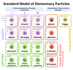 | |||||||
| Constituents |
| ||||||||
| Beyond theStandard Model |
| ||||||||
| Experiments |
|